# Machine Learning Over Streaming Kafka® Data—Part 2: Introduction to Batch Training and TensorFlow
[Blog](/blog/)>[Technology](/blog/category/technical/)>Machine Learning Over Streaming Kafka® Data—Part 2: Introduction to Batch Training and TensorFlow
Machine Learning Over Streaming Kafka® Data—Part 2: Introduction to Batch Training and TensorFlow
=================================================================================================
July 26, 2023 | By [ Paul Brebner](https://www.instaclustr.com/blog/author/paul-brebner/)
[ ](https://x.com/intent/tweet?text=Machine%20Learning%20Over%20Streaming%20Kafka%C2%AE%20Data%E2%80%94Part%202:%20Introduction%20to%20Batch%20Training%20and%20TensorFlow&url=https://www.instaclustr.com/blog/machine-learning-over-streaming-kafka-data-part-2/) [ ](https://www.linkedin.com/shareArticle?mini=true&url=https://www.instaclustr.com/blog/machine-learning-over-streaming-kafka-data-part-2/&title=&summary=Machine%20Learning%20Over%20Streaming%20Kafka%C2%AE%20Data%E2%80%94Part%202:%20Introduction%20to%20Batch%20Training%20and%20TensorFlow&source=)
As I mentioned in [Part 1](https://www.instaclustr.com/blog/machine-learning-over-streaming-apache-kafka-data-part-1-introduction/) of this series, we are looking at Machine Learning (ML) over streaming Apache Kafka® data. But rather than just jumping in—and immediately going over a fast-flowing waterfall (in a barrel, which people have actually attempted!)—I first need to get a good understanding of TensorFlow with some “still” (static and unchanging) data and batch learning to start with. This will be easier and repeatable before we encounter Kafka and streaming and changing data.
[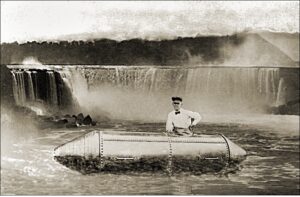](https://www.instaclustr.com/wp-content/uploads/2023/07/Niaga-Falls-Daredevil.jpg)Niagra Falls Daredevil—I assume he was one of the few survivors—unless this was a publicity photo before he went over the falls. (Source: Shutterstock)
In this blog you will learn the basic steps for batch learning over static data with TensorFlow, including how to set up a Python TensorFlow environment, importing pandas and numpies, defining the data columns and the learning class, reading the data into a Panda DataFrame, splitting the data into training/evaluation sets, creating a model, and training and evaluating the model.
Experiment 1: Batch Processing With TensorFlow
------------------------------------------------
Here’s the basic TensorFlow batch code, designed to use 1 week of [drone delivery data](https://www.instaclustr.com/blog/spinning-your-drones-with-cadence-introduction-part-3/). Oh, and watch out—it’s in Python (a programming language I’m no expert in).
First, you have to set up a Python and TensorFlow environment on your computer. I followed [these instructions](https://www.tensorflow.org/install) with the addition of the following extra commands:
python3 -m pip install --upgrade pip pip install scikit-learn pip install pandas <span data-ccp-props="{}"> </span>
1
2
3
4
5
python3 -m pip install --upgrade pip
pip install scikit-learn
pip install pandas <span data-ccp-props="{}"> </span>
Then there is a series of steps required, including
- Reading the file into an internal data structure
- Defining columns and which one is the class to be learned
- Splitting the data into training and test data subsets
- Defining and compiling a model (which is initially untrained), and finally
- Training and then evaluating the model.
Now, here are the basic steps using the example Python code from above:
1. ### Import Pandas and Nump(t)ies
[](https://www.instaclustr.com/wp-content/uploads/2023/07/Numpty.jpg)My word processor wanted to autocorrect “numpy” to “Numpty”—an alteration of numbskull, with the ending remodeled on the pattern of Humpty Dumpty (Source: Shutterstock)
First, import pandas and numpies (2 weird-sounding things I’ll explain more in detail below)
import os from datetime import datetime import time import threading import json from sklearn.model\_selection import train\_test\_split import pandas as pd import numpy as np import tensorflow as tf import tensorflow\_io as tfio
1
2
3
4
5
6
7
8
9
10
11
12
13
14
15
16
17
18
19
import os
from datetime import datetime
import time
import threading
import json
from sklearn.model\_selection import train\_test\_split
import pandas as pd
import numpy as np
import tensorflow as tf
import tensorflow\_io as tfio
2. ### Define Columns
Next, define the columns that the CSV data has. In my case, the first column is the ‘class’ that is to be learned. The label (if a shop is busy or not busy in a given hour), and the rest are features (we have 5 extra randomly generated features just to add some complexity):
\# define data columns
DCOLUMNS = \[ # labels 'class', 'shop\_id', 'shop\_type', 'shop\_location', 'weekday', 'hour', 'avgTime', 'avgDistance', 'avgRating', 'another1', 'another2', 'another3', 'another4', 'another5' \]
1
2
3
4
5
6
7
8
9
10
11
12
13
14
15
16
17
18
19
20
21
22
23
24
25
26
27
28
29
30
31
32
33
DCOLUMNS = \[
\# labels
'class',
'shop\_id',
'shop\_type',
'shop\_location',
'weekday',
'hour',
'avgTime',
'avgDistance',
'avgRating',
'another1',
'another2',
'another3',
'another4',
'another5'
\]
3. ### Read the File into Pandas
[](https://www.instaclustr.com/wp-content/uploads/2023/07/Panda.jpg)
*(Source: Shutterstock)*
Next, read the CSV file into a panda data type. A Panda [DataFrame](https://pandas.pydata.org/docs/user_guide/dsintro.html#basics-dataframe) is just a 2-dimensional, size-mutable, potentially heterogeneous tabular data structure—basically just a 2d array I suspect.
For these, I borrowed some code from [here](https://www.tensorflow.org/tutorials/load_data/pandas_dataframe):
\# read csv file fname = 'week1.csv' drone\_iterator = pd.read\_csv(fname, header=None, names=DCOLUMNS, chunksize=100000) drone\_df = next(drone\_iterator) print(drone\_df.head()) print("size ", drone\_df.size) print("data types ", drone\_df.dtypes) l1 = len(drone\_df) l2 = len(drone\_df.columns) l3 = len(drone\_df\[drone\_df\["class"\]==0\]) l4 = len(drone\_df\[drone\_df\["class"\]==1\]) print("records ", l1, " columns ", l2, " class 0 ", l3, " class 1 ", l4) NUM\_COLUMNS = len(drone\_df.columns)
1
2
3
4
5
6
7
8
9
10
11
12
13
14
15
16
17
18
19
20
21
22
23
24
25
26
27
\# read csv file
fname = 'week1.csv'
drone\_iterator = pd.read\_csv(fname, header=None, names=DCOLUMNS, chunksize=100000)
drone\_df = next(drone\_iterator)
print(drone\_df.head())
print("size ", drone\_df.size)
print("data types ", drone\_df.dtypes)
l1 = len(drone\_df)
l2 = len(drone\_df.columns)
l3 = len(drone\_df\[drone\_df\["class"\]==0\])
l4 = len(drone\_df\[drone\_df\["class"\]==1\])
print("records ", l1, " columns ", l2, " class 0 ", l3, " class 1 ", l4)
NUM\_COLUMNS = len(drone\_df.columns)
4. ### Split the Data
[](https://www.instaclustr.com/wp-content/uploads/2023/07/Log.jpg)
*(Source: Shutterstock)*
Next, we need to split the data into 2 subsets—one for training and one for evaluation. If you use all the data for training, you will potentially overfit the model. If that happens, it won’t work as well for new unseen observations, and you also won’t have any data left over for evaluation:
\# split the data into training and test sets train\_df, test\_df = train\_test\_split(drone\_df, test\_size=0.4, shuffle=True) print("Number of training samples: ",len(train\_df)) print("Number of testing samples: ",len(test\_df)) print(train\_df.head()) print(test\_df.head())
1
2
3
4
5
6
7
8
9
10
11
12
13
14
15
\# split the data into training and test sets
train\_df, test\_df = train\_test\_split(drone\_df, test\_size=0.4, shuffle=True)
print("Number of training samples: ",len(train\_df))
print("Number of testing samples: ",len(test\_df))
print(train\_df.head())
print(test\_df.head())
The “train\_test\_split” function takes arguments including the data to split, the ratio to use for test data, and whether to shuffle the data to make the split or not—if you don’t shuffle it, then it will simply take the first 60% for training and the last 40% for testing for this example.
5. ### Create a Model With the Adam Optimizer
[](https://www.instaclustr.com/wp-content/uploads/2023/07/Creation-of-Adam.png)The creation of Adam—by a Robot (by an AI – custom image via Paul Brebner and Dalle-E)
Next, we need to design, build and compile a model:
\# design the model # Set the parameters OPTIMIZER="adam" LOSS=tf.keras.losses.BinaryCrossentropy(from\_logits=True) METRICS=\['accuracy', tf.keras.metrics.TruePositives(), tf.keras.metrics.TrueNegatives(), tf.keras.metrics.FalsePositives(), tf.keras.metrics.FalseNegatives()\] # 32 is the default batch size BATCH\_SIZE=32 # EPOCHS is the number of times to train with each batch of data EPOCHS=200 # design/build the model model = tf.keras.Sequential(\[ tf.keras.layers.Input(shape=(NUM\_COLUMNS,)), tf.keras.layers.Dense(128, activation='relu'), tf.keras.layers.Dropout(0.2), tf.keras.layers.Dense(256, activation='relu'), tf.keras.layers.Dropout(0.4), tf.keras.layers.Dense(128, activation='relu'), tf.keras.layers.Dropout(0.4), tf.keras.layers.Dense(1, activation='sigmoid') \]) print(model.summary()) # compile the model model.compile(optimizer=OPTIMIZER, loss=LOSS, metrics=METRICS)
1
2
3
4
5
6
7
8
9
10
11
12
13
14
15
16
17
18
19
20
21
22
23
24
25
26
27
28
29
30
31
32
33
34
35
36
37
38
39
40
41
42
43
44
45
46
47
48
49
50
51
52
53
\# design the model
\# Set the parameters
OPTIMIZER="adam"
LOSS=tf.keras.losses.BinaryCrossentropy(from\_logits=True)
METRICS=\['accuracy', tf.keras.metrics.TruePositives(), tf.keras.metrics.TrueNegatives(), tf.keras.metrics.FalsePositives(), tf.keras.metrics.FalseNegatives()\]
\# 32 is the default batch size
BATCH\_SIZE=32
\# EPOCHS is the number of times to train with each batch of data
EPOCHS=200
\# design/build the model
model = tf.keras.Sequential(\[
tf.keras.layers.Input(shape=(NUM\_COLUMNS,)),
tf.keras.layers.Dense(128, activation='relu'),
tf.keras.layers.Dropout(0.2),
tf.keras.layers.Dense(256, activation='relu'),
tf.keras.layers.Dropout(0.4),
tf.keras.layers.Dense(128, activation='relu'),
tf.keras.layers.Dropout(0.4),
tf.keras.layers.Dense(1, activation='sigmoid')
\])
print(model.summary())
\# compile the model
model.compile(optimizer=OPTIMIZER, loss=LOSS, metrics=METRICS)
As you can see, many weird and wonderful settings are required—this one used the [Adam algorithm](https://www.tensorflow.org/api_docs/python/tf/keras/optimizers/Adam). Fun fact: the Adam algorithm actually has nothing to do with Adam and Eve; instead, [the name Adam](https://machinelearningmastery.com/adam-optimization-algorithm-for-deep-learning/) is derived from “adaptive moment estimation”.
Batch size and Epoch are important concepts and correspond to the number of observations used at once for training, and the number of iterations to train the model.
6. ### Train/Fit the Model
[](https://www.instaclustr.com/wp-content/uploads/2023/07/Mouse.jpg)Bodybuilding training is all about the Reps (repetitions) = Epochs (Source: Shutterstock)
Next, we must get the data ready for training – and then actually train it by calling “fit”:
\# get data ready for training drone\_features = train\_df.copy() drone\_labels = drone\_features.pop('class') drone\_features = np.array(drone\_features)
1
2
3
4
5
6
7
\# get data ready for training
drone\_features = train\_df.copy()
drone\_labels = drone\_features.pop('class')
drone\_features = np.array(drone\_features)
\# rather than a fixed number of epochs, it’s better to allow the model to stop when a metric stops improving for patience number of epochs
callback = tf.keras.callbacks.EarlyStopping(monitor='accuracy', patience=10)
1
callback = tf.keras.callbacks.EarlyStopping(monitor='accuracy', patience=10)
model.fit(drone\_features, drone\_labels, batch\_size=BATCH\_SIZE, epochs=EPOCHS, callbacks=\[callback\])
1
model.fit(drone\_features, drone\_labels, batch\_size=BATCH\_SIZE, epochs=EPOCHS, callbacks=\[callback\])
The fit method needs 2 DataFrames: the first containing the features only, and the second containing the labels (the class to be learned). We prepare 2 DataFrames, drone\_labels and drone\_features for this. Drone\_features is created using the NumPy library (NumPy is the fundamental package for scientific computing in Python—the fundamental NumPy datatype is an n-dimensional arrays of homogeneous data types).
The other important trick here is that rather than calling fit with a fixed number of Epochs, we define a callback which stops learning whenever a condition is met—in this case the accuracy doesn’t improve for 10 iterations. I discovered that this can significantly improve the accuracy of the training and reduce the training time if the training occurs faster than expected.
Another thing to note is that every time the fit method is called, the model is updated with the data provided—by default it doesn’t start training from scratch each time
7. ### Evaluate the Model
Now it’s time to see how well the model performed on the data we left over for testing—we must prepare it as for the training data, and then call the evaluate method:
\# prepare the test data for evaluation drone\_features\_test = test\_df.copy() drone\_labels\_test = drone\_features\_test.pop('class') drone\_features\_test = np.array(drone\_features\_test) print('testing...') print(model.evaluate(drone\_features\_test, drone\_labels\_test))
1
2
3
4
5
6
7
8
9
10
11
12
13
14
\# prepare the test data for evaluation
drone\_features\_test = test\_df.copy()
drone\_labels\_test = drone\_features\_test.pop('class')
drone\_features\_test = np.array(drone\_features\_test)
print('testing...')
print(model.evaluate(drone\_features\_test, drone\_labels\_test))
So, there we have the basic steps for batch learning with TensorFlow.
But how did this all perform/work out? I certainly had a few hypotheses myself, but even I was a bit surprised at what unfurled.
In [the next part](https://www.instaclustr.com/blog/machine-learning-over-streaming-kafka-data-part-3-introduction-to-batch-training-and-tensorflow-results/), we’ll explore performance metrics, show an example trace—and find out how long training actually takes.
Follow the series: Machine Learning Over Streaming Kafka® Data
--------------------------------------------------------------
**[Part 1: Introduction](https://www.instaclustr.com/blog/machine-learning-over-streaming-apache-kafka-data-part-1-introduction/)**
[Part 2: Introduction to Batch Training and TensorFlow](https://www.instaclustr.com/blog/machine-learning-over-streaming-kafka-data-part-2/)
[**Part 3: Introduction to Batch Training and TensorFlow Results**](https://www.instaclustr.com/blog/machine-learning-over-streaming-kafka-data-part-3-introduction-to-batch-training-and-tensorflow-results/)
[**Part 4: Introduction to Incremental Training With TensorFlow**](https://www.instaclustr.com/blog/machine-learning-over-streaming-kafka-data-part-4-introduction-to-incremental-training-with-tensorflow/)
**[Part 5: Incremental TensorFlow Training With Kafka Data](https://www.instaclustr.com/blog/machine-learning-over-streaming-kafka-data-part-5-incremental-tensorflow-training-with-kafka-data/)**
**[Part 6: Incremental TensorFlow Training With Kafka Data and Concept Drift](https://www.instaclustr.com/blog/machine-learning-over-streaming-kafka-data-part-6-incremental-tensorflow-training-with-kafka-data-and-concept-drift/)**
### About the author
**[Paul Brebner](https://www.instaclustr.com/blog/author/paul-brebner/)** | Technology Evangelist at Instaclustr
Paul has extensive R&D and consulting experience in distributed systems, technology innovation, software architecture, and engineering, software performance and scalability, grid and cloud computing, and data analytics and machine learning.
![mail icon]()#### Get the latest articles for open sourceIn your inbox
### Related content
[ Third Contact With a Monolith—Beam Me Down Scotty
This is the third of the four-part series of "Contact with Monolith" by Paul Brebner, Tech. Evangelist at Instaclustr...
](https://www.instaclustr.com/blog/third-contact-monolith-beam-scotty/)
[ Airflow vs Cadence: A Side-by-Side Comparison
Apache Airflow and Cadence are both workflow management ecosystems, it is important for developers to know which solutions are ...
](https://www.instaclustr.com/blog/airflow-vs-cadence-a-side-to-side-comparison/)
[ Apache Kafka “Kongo” Part 4.1: Connecting Kafka to Cassandra with Kafka Connect
Use case extending the Kongo IoT application to stream events from Kafka to Cassandra using a Kafka Connect Cassandra Sink...
](https://www.instaclustr.com/blog/apache-kafka-kongo-part-4-1-connecting-kafka-cassandra-kafka-connect/)
×Sign upto ourNewsletter
-----------------------