OpenSearch 3.0 Dashboards offer an incredible range of tools to help you visualize complex datasets. Whether you’re analyzing web traffic, monitoring logs, or uncovering trends, advanced visualization types like Vega, VisBuilder, and TSVB (Time Series Visual Builder) take your dashboards to the next level. This step-by-step guide will walk you through each tool, demonstrating how to use OpenSearch dashboards effectively to make data interpretation easier and more impactful.
In previous posts (like this one), I’ve covered exploring and creating basic visualizations in OpenSearch 3.0 Dashboards. Now I’ll dive a little deeper into the more complex visualization types in OpenSearch Dashboards
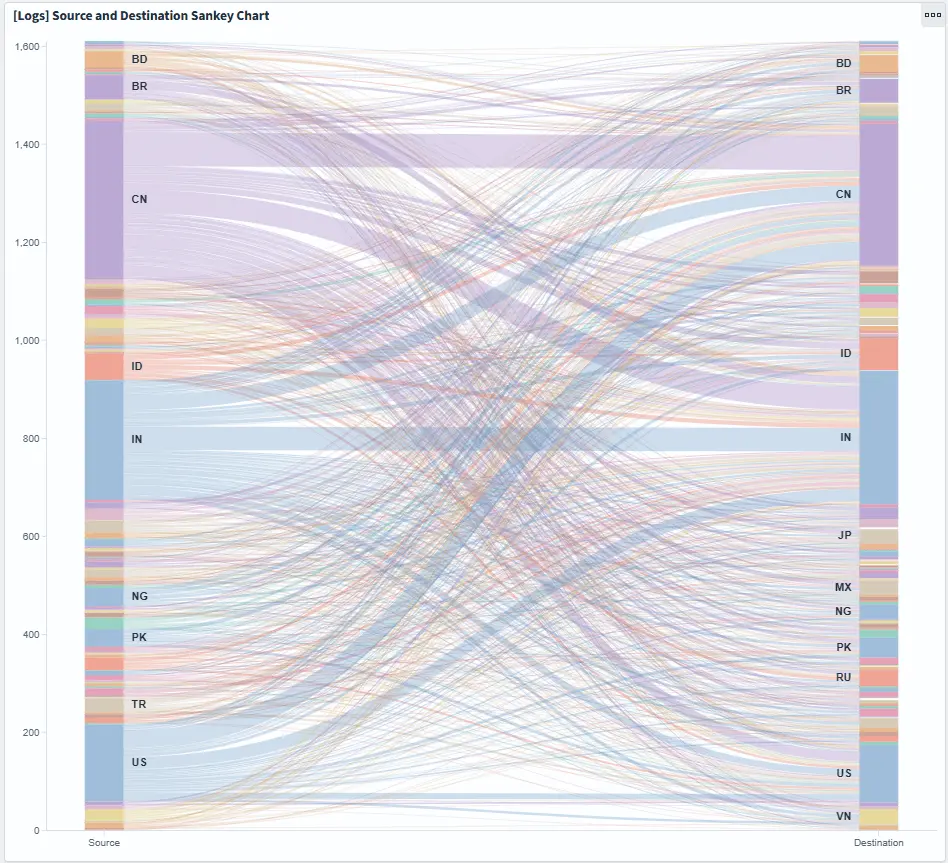
Some of these visualization types open powerful options but require users to learn a new declarative language (Vega or Vega-Lite). However, some of these tools can also be easy-to-understand and allow you to visually build visualizations (VisBuilder). In the middle you have the TSVB, which allows you to create a marked-up timeline of events in your OpenSearch data. These types of visualizations can be useful for advanced displays like the Sankey chart below in the Vega section, and time series data like logs for incident monitoring and reporting.
Now why would you want to go to all the trouble of creating advanced visualizations? There are some very strong real-world cases: if you’d like to see web request logs in more facets, you can create things like Sankey charts for origin-to-destination mapping or create line graphs that separate the requests by response code. Some of these tools, like the VisBuilder, are powerful yet offer a user experience that makes creating even advanced charts easier. These advanced charts can help you visualize even the most complicated of data in a way that more people can understand.
Now I’ll cover each type in detail, including when to use it, how to use it, and how to create a visualization with it.
Vega/Vega-Lite
Vega and its counterpart Vega-Lite can be a bit intimidating to use at first; these are declarative, JSON-based languages that allow you to declare all parts of a visualization. Vega and Vega-Lite are the heavy-hitters: if you have a visualization that you cannot find out-of-the-box in OpenSearch Dashboards, you’ll want to take a look at the Vega and Vega-Lite docs, and the Vega/Vega-Lite OpenSearch Dashboards docs.
It’s also well-explained in the Vega example in the comments: “In Vega, you have the full control of what data is loaded, even from multiple sources, how that data is transformed, and what visual elements are used to show it.”
Vega-Lite was used to create the Sankey chart on the Web Logs dashboard in the OpenSearch pre-loaded data:
You’re going to build something a bit simpler: an average bytes over time graph.
If you aren’t following along from my previous post, you can use the instructions there to either spin up a free trial of a NetApp Instaclustr OpenSearch 3.0 preview cluster, or you can use the OpenSearch Dashboards Playground to follow along. Use the web traffic data if spinning up OpenSearch 3.0 on NetApp Instaclustr.
Building a Vega/Vega-Lite visualization
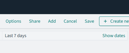
First, you’ll want to create a new Dashboard, and click Edit in the upper right corner:
Then the Edit button will turn into a Create new button.
Click it to see the menu of choices for panel visualizations:

Select Vega. You’ll be taken to an editing screen:
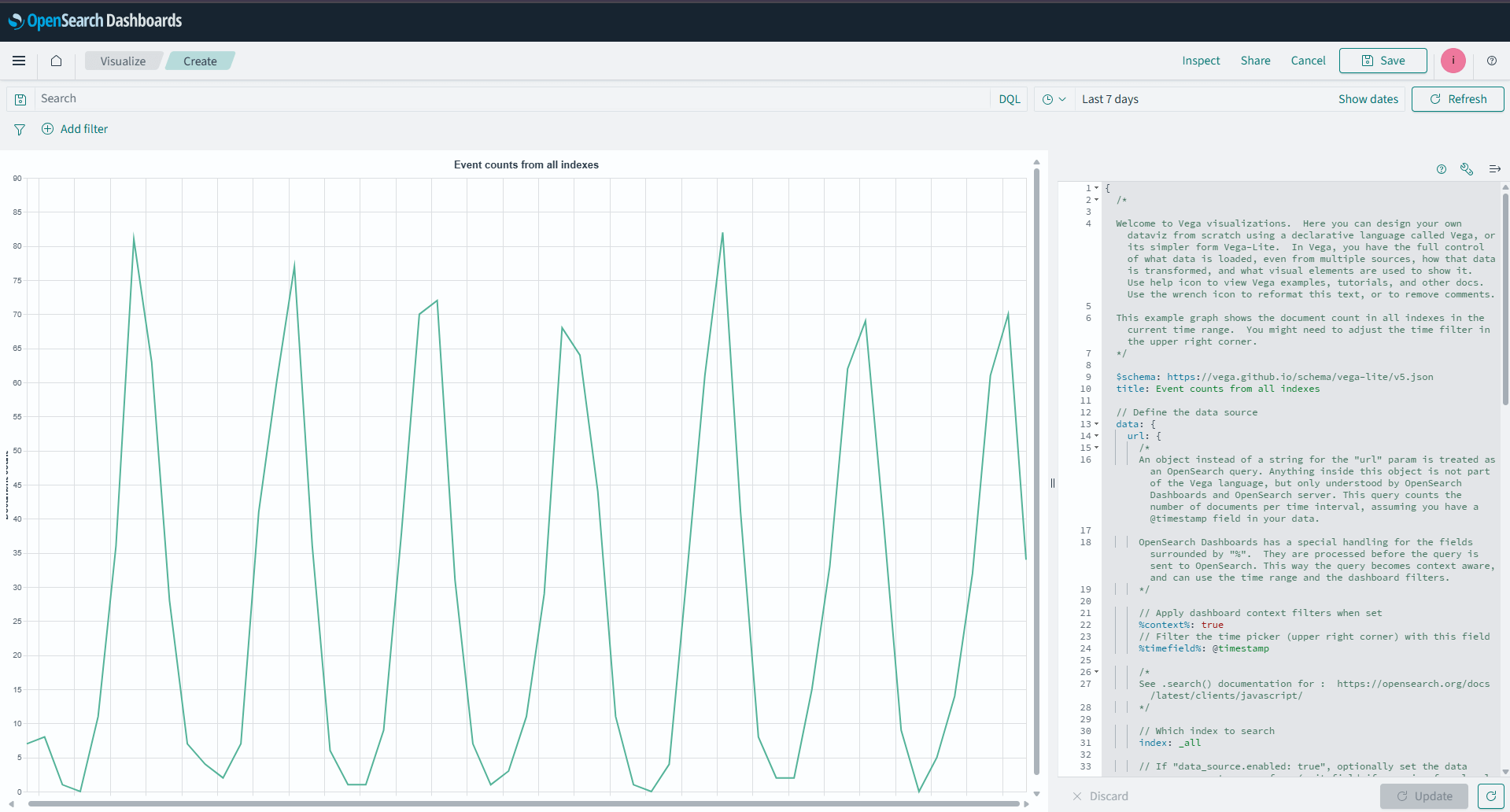
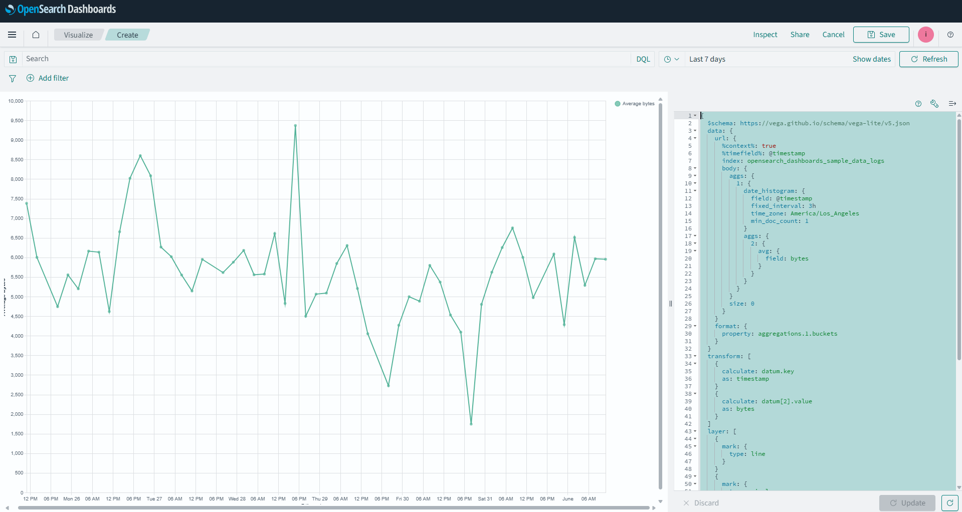
Luckily, you’re not greeted with a blank slate: there’s a line chart of events over time. You’re going to explore the Vega and edit it to show average bytes over time. To do this, we’ll need to edit the data bucket that the Vega visualization pulls from. Replace the code in the visualization panel with the following:
|
1 2 3 4 5 6 7 8 9 10 11 12 13 14 15 16 17 18 19 20 21 22 23 24 25 26 27 28 29 30 31 32 33 34 35 36 37 38 39 40 41 42 43 44 45 46 47 48 49 50 51 52 53 54 55 56 57 58 59 60 61 62 63 64 65 66 67 68 69 70 71 72 73 74 75 76 77 78 79 80 81 82 83 |
{ $schema: https://vega.github.io/schema/vega-lite/v5.json data: { url: { %context%: true %timefield%: @timestamp /* tells the visualization which index to use */ index: opensearch_dashboards_sample_data_logs /* This sets up the buckets used for X and Y axis values */ body: { /* Sets up 2 aggregation buckets... */ aggs: { 1: { /* ...one for the timestamps for the X axis... */ date_histogram: { field: @timestamp fixed_interval: 3h time_zone: America/Los_Angeles min_doc_count: 1 } /* ... and one for the bytes sent in that time frame */ aggs: { 2: { avg: { field: bytes } } } } } size: 0 } } format: { property: aggregations.1.buckets } } transform: [ { /* you can transform your data here. In this case, we are just mapping to the timestanmps and the average bytes */ calculate: datum.key as: timestamp } { calculate: datum[2].value as: bytes } ] layer: [ { mark: { type: line } } { mark: { type: circle tooltip: true } } ] /* Now that we've set up the buckets and transformed (set) the data points, you'll tell the graph how to map each axis. */ encoding: { x: { field: timestamp type: temporal axis: { title: @timestamp } } y: { field: bytes type: quantitative axis: { title: Average bytes } } color: { datum: Average bytes type: nominal } } } |
(You can also copy the code from this gist). This creates an average bytes over time visualization.
Hit the Update button at the bottom to see your new graph:
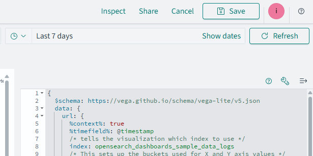
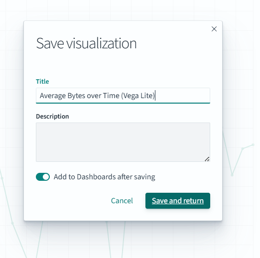
Click the Save button at the top right to save your new Vega lite visualization.
You’ll see a pop-up to name your visualization. Name it “Average Bytes over Time (Vega lite)” and make sure Add to Dashboards after saving is checked. Then, hit Save and return.
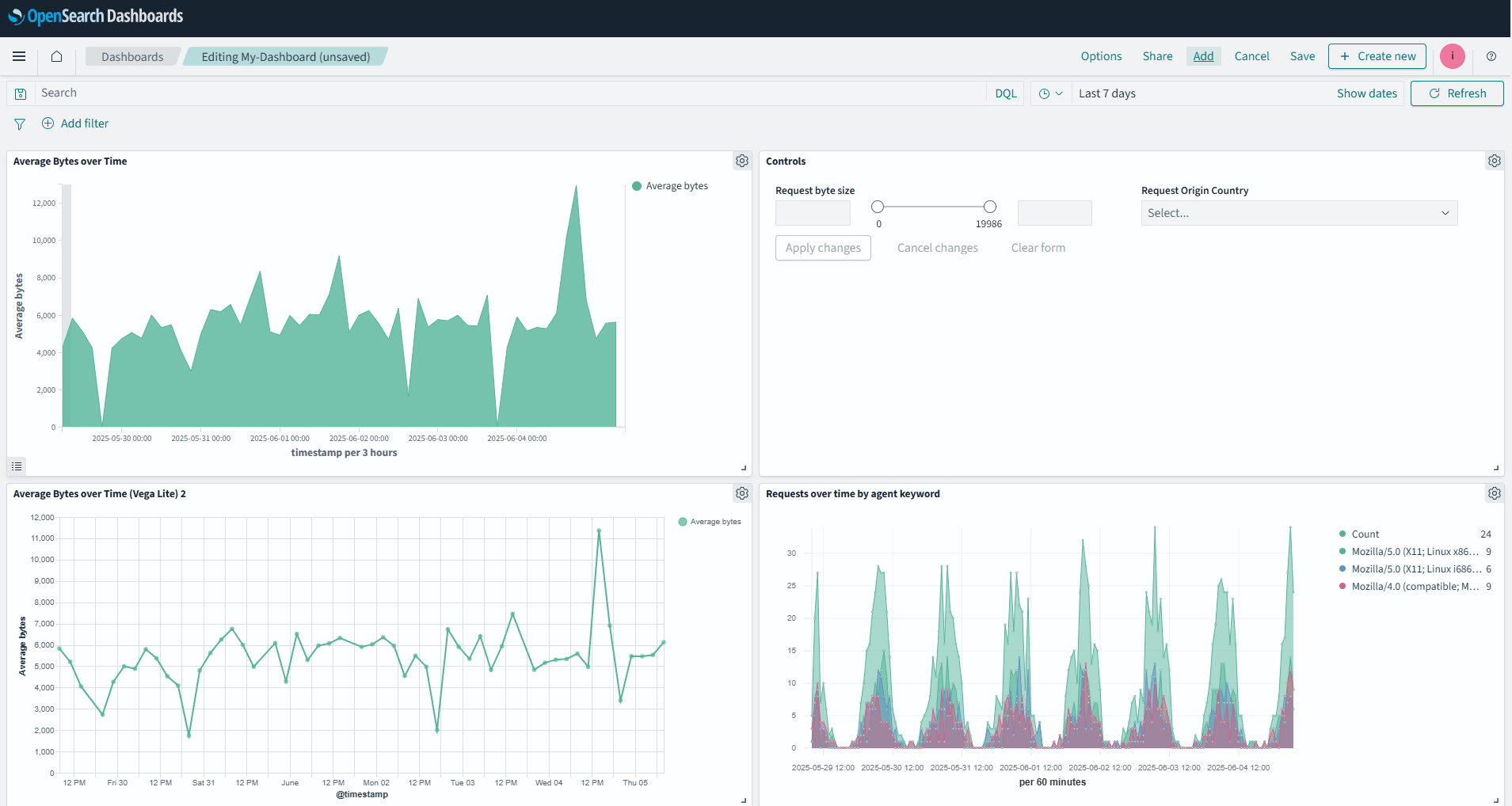
You’ll be taken back to your dashboard; if you followed along last post, it’ll look like this:
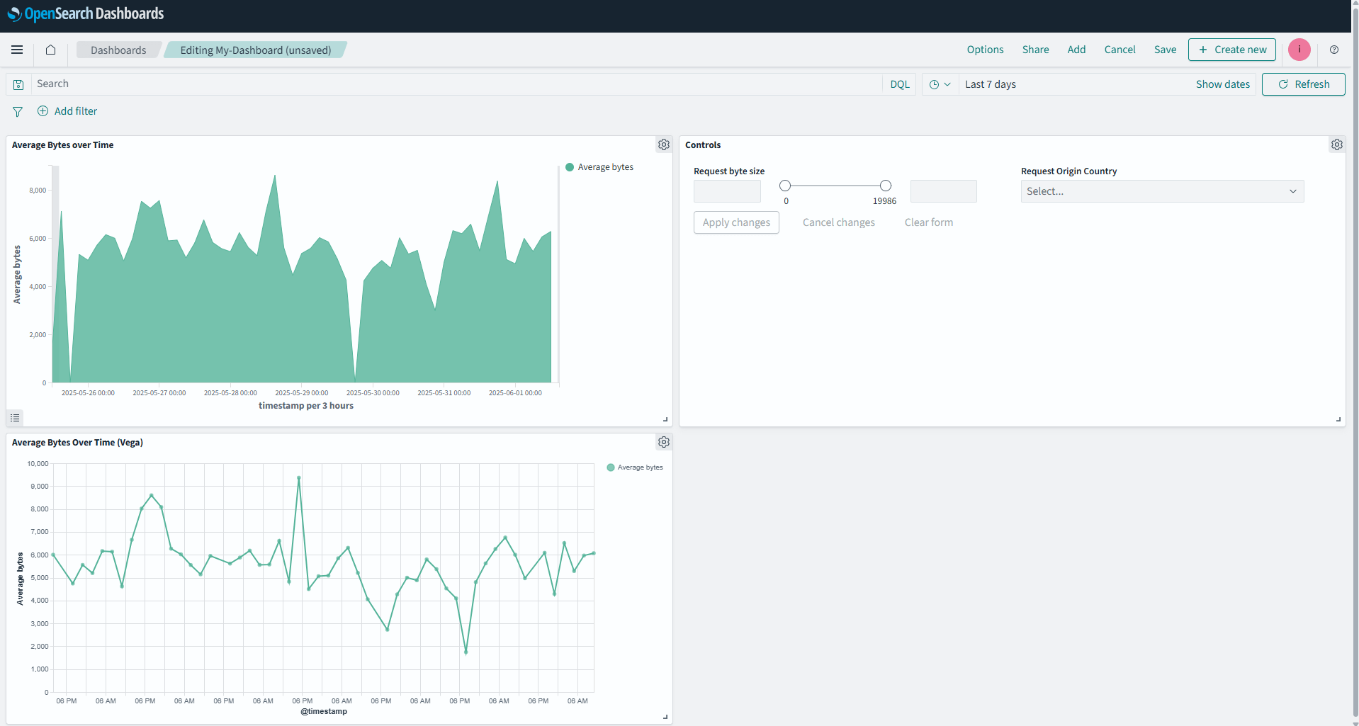
You can see your new Vega visualization in the lower left. Now make sure you save your dashboard using the Save link on the upper right:
You can do a lot more with Vega and Vega-Lite; from tooltips to custom labels to entirely new visualizations. Next, you’ll look at the VisBuilder, a bit more intuitive way of creating new visualizations.
VisBuilder
VisBuilder is interesting in that while it can create some advanced visualizations, it does so with a drag and drop interface. You’ll start at your Dashboard, click the Edit button at the top right, then Create new in the same place. Select VisBuilder from the menu. You’ll be greeted with the following interface:
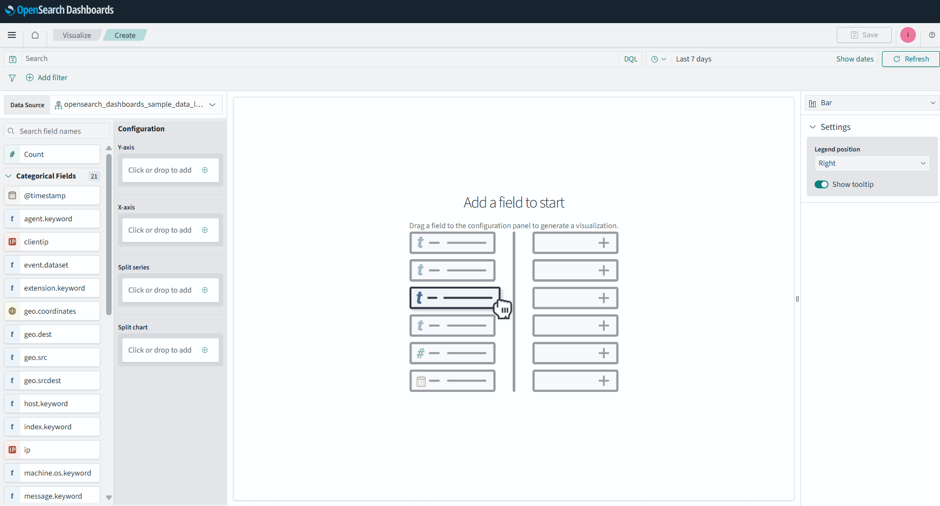
You’re going to use this to build a stacked graph of average requests and bytes over time. To start, you need a value for your X-axis. We want to use a timestamp field, so drag the @timestamp field over to the X-axis bucket:
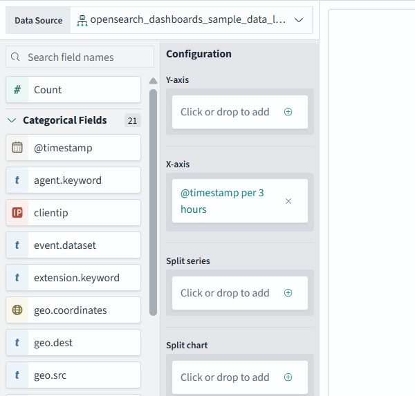
It’ll pop up a warning about needing an aggregate. We’ll add the average bytes by dragging the bytes item (under Numerical Fields) into the Y-axis bucket:
Next, you’ll add the second aggregate, the number of requests. To do this, scroll to the top of the list at the left, and drag Count and add it to the Y-axis bin:
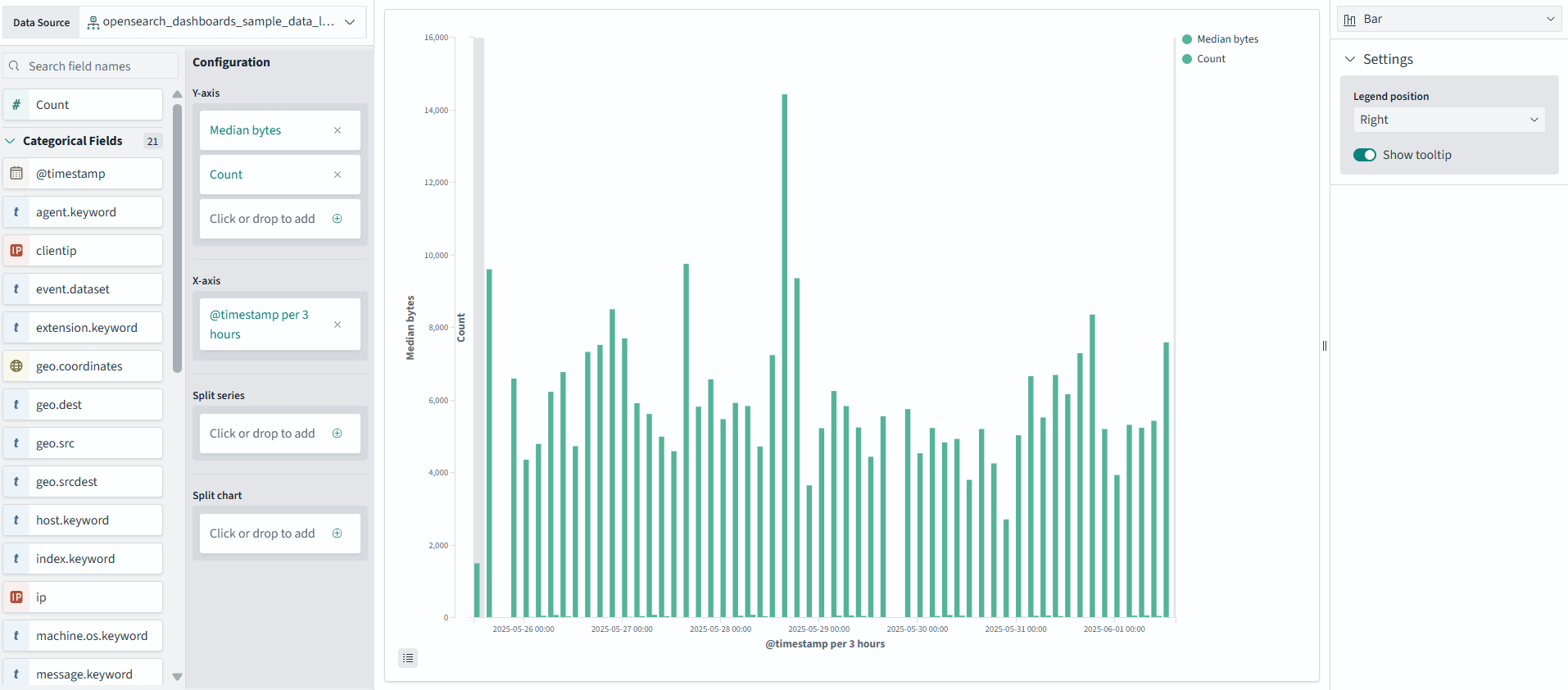
It’s a little hard to see the count because of the format of the graph and the disparity of the values. You’ll change this by first changing the color of count by clicking the little green circle next to the Count label in the graph legend:
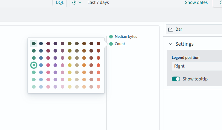
Pick any other color and it will stand out a bit more.
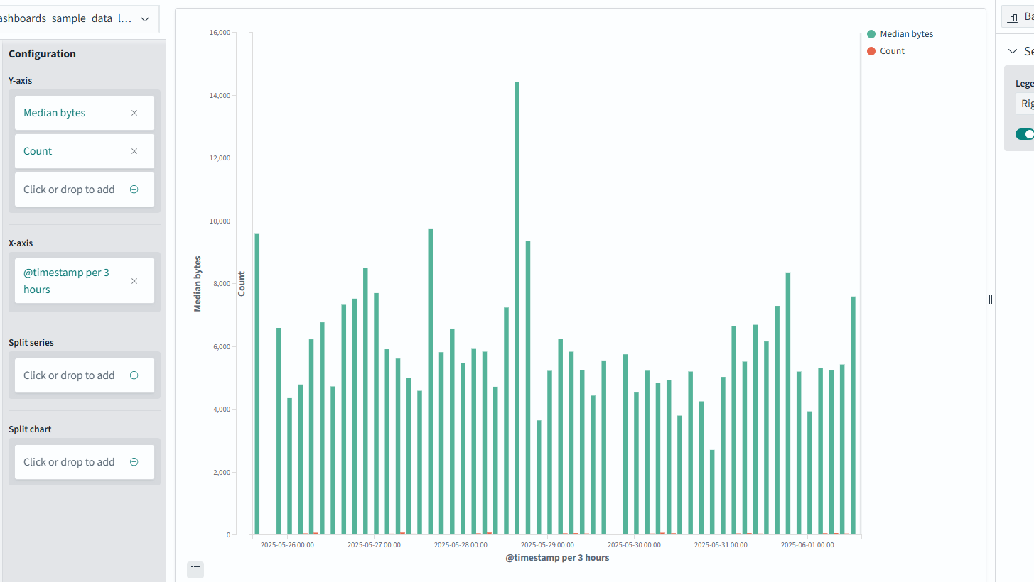
The last thing you’ll do to help differentiate is by turning it into an area chart. On the top of the right panel is a dropdown to change the type of visualization:
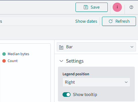
Click this dropdown, then select Area (Bar is selected by default):
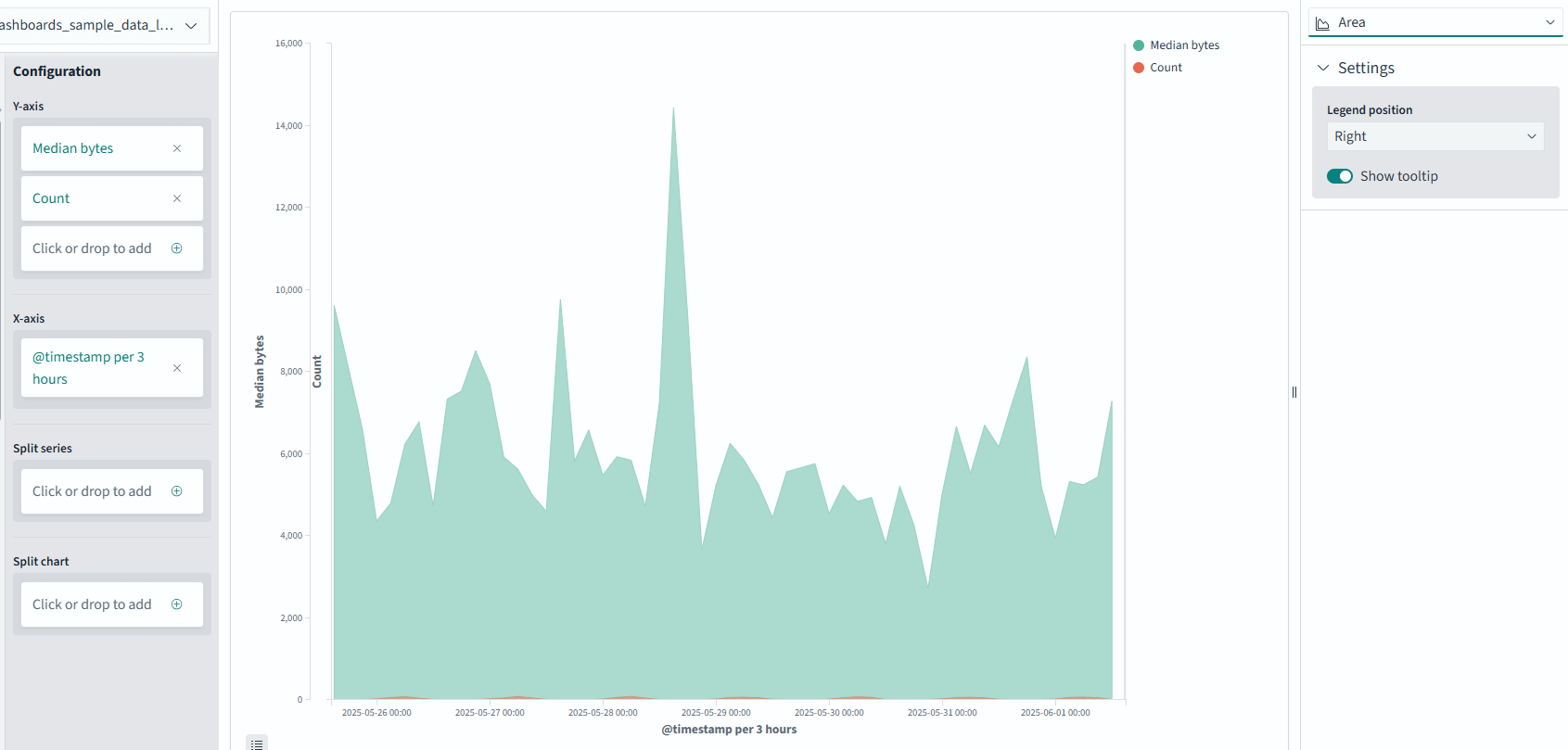
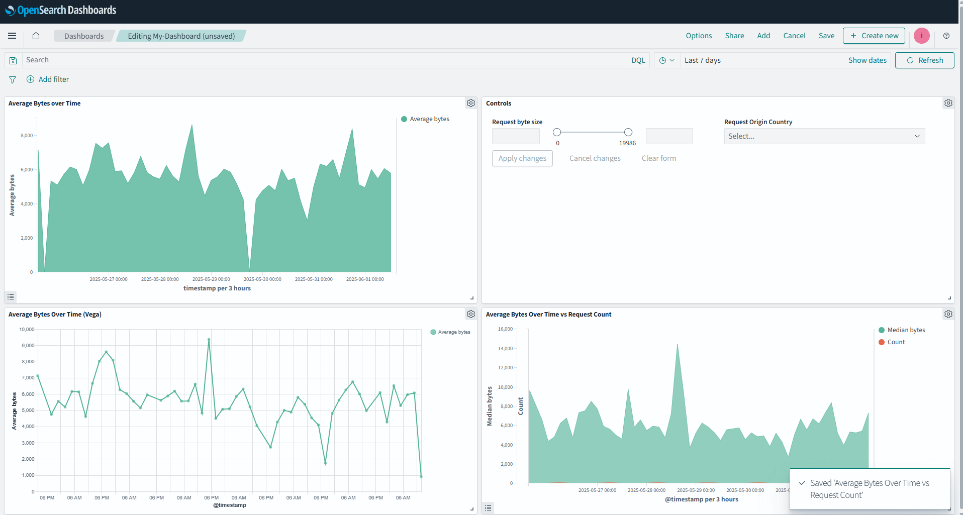
You can use graphs like this to map correlations between data sets. Make sure to save your visualization (I named it “Average Bytes Over Time vs Request Count”) and you’ll see it on the dashboard:
Save your dashboard using the save button on the top right, and you’ll be ready to tackle the last type of advanced visualizations in this post; TSVB, or Time Series Visualization Builder.
TSVB (Time Series Visualization Builder)
The TSVB is great for timeline series data that you want to annotate and visualize. While you can build tables, gauges, and Markdown panels with this tool, I’ll stick to the timeline builder for this example. Select Create new on the upper left of your Dashboard and select TSVB from the dialog box.
You’ll be greeted with something like this:
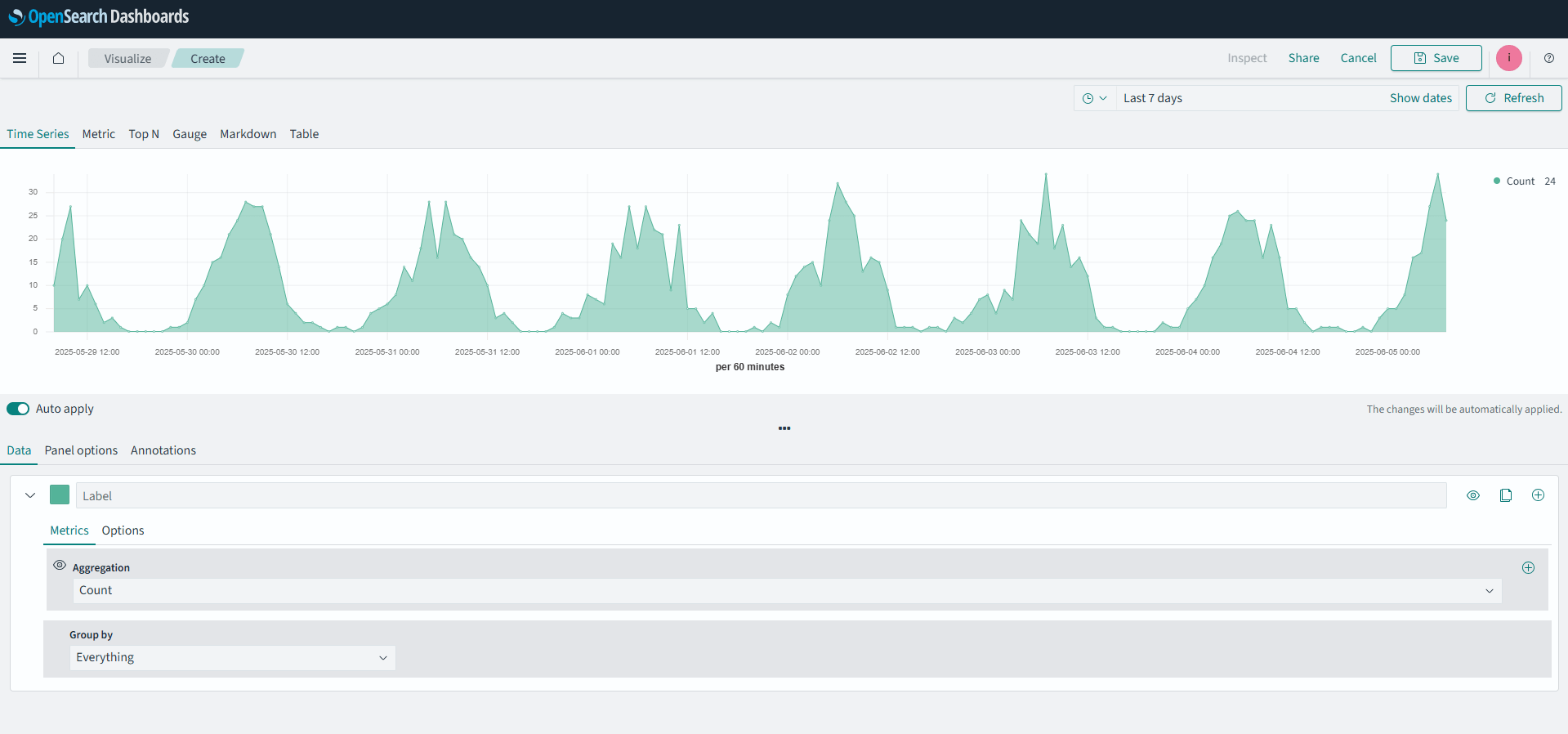
This is a timeline of request counts over time. You’re going to add another data; those same requests separated by agent.keyword (the browser agent the request came from).
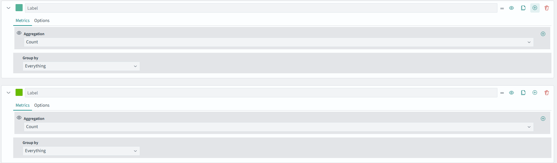
In the lower panel of the screen, where it says label, go to the right and you’ll see an Add (+) button:
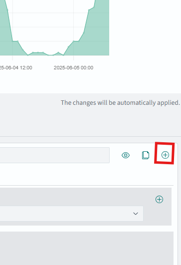
Click it, and a second label will made and appear below the default one.
In the new label, change the Group by dropdown to Terms. This will pop up some new options:
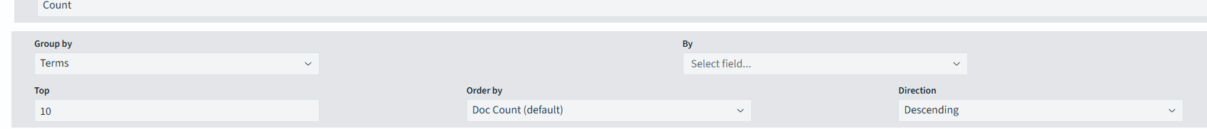
Change By to agent.keyword. Your datum should look like this:

Finally, your visualization should look like this:

Hit Save and add it to your dashboard:
And there you have it, a quick dive into three of the more powerful visualization types in OpenSearch 3.0 Dashboards: the Vega/Vega-Lite, VisBuilder, and TSVB.
Final thoughts
Creating advanced visualizations in OpenSearch dashboards doesn’t have to be daunting. With tools like Vega, VisBuilder, and TSVB, you can handle everything from basic comparisons to rich, interactive datasets that drive better decisions.
Start building your optimized dashboards today, and make sure to try out the free OpenSearch 3.0 trial on NetApp Instaclustr to follow along, and you can always read more on the Instaclustr blog.
Your data has stories to tell; OpenSearch dashboards help you tell them.