Quick! Grab your top hat, passport, carpetbag stuffed with (mainly) cash, and your valet (if you have one), and join with me on a wild journey around the world in approximately 8 data centers—a new blog series to explore the world of globally distributed storage, streaming, and search with Instaclustr Managed Open Source Technologies such as Apache Cassandra and Apache Kafka.

Around The World In 80 Days (Source: Shutterstock)
In this new blog series, we’ll explore globally distributed applications in the context of Cloud Location, including many of the drivers and concerns such as correctness and replication (making sure applications work correctly by having the data they need in the correct locations), latency (reducing lag for end-users), redundancy and replication (making sure applications are available even if an entire data center fails), cost (understanding how much it costs to run an application in multiple locations, and if the cost can be reduced), and data sovereignty (ensuring customer data is only stored in legal locations). Surprisingly, Jules Verne captured these elements in Around the World: correctness (proof that they traveled around the world), time (80 days, and selecting locations and routes to travel around the world in the allotted time), success and failure (the wager), money (half Fogg’s fortune was in the carpetbag), and sovereignty (as Detective Fix repeatedly tries to arrest them at locations in the British Empire). By the end of this first blog I wager we’ll have answered our first question of the series: “How many data centers do you need for a globally distributed application?”
1. Where Are the Clouds?
Is there anything wrong with this image of the Earth?
 (Source: Shutterstock)
Yes, it’s “too perfect”, it’s fake! It’s called the “Blue Marble” view of the Earth and (impossibly) it doesn’t have any clouds. Did you know that 67 per cent of Earth’s surface is typically covered by clouds? But clouds are more common in some regions than others (see cloud map below – dark blue = cloud uncommon, white = cloud common), so clouds obscure the view from space more often than not in many parts of the world, making it tricky to get cloud-free photos (image processing of multiple photos is used to create a cloud-free photo).

https://earthobservatory.nasa.gov/images/85843/cloudy-earth
Cleverly, some scientists used the original satellite imagery (with clouds) to create maps that reveal things about the underlying ecosystems of the planet, for example, to accurately map the boundaries of continuously cloudy regions which are home to “cloud forests” (unique high-elevation ecosystems known for harboring remarkable biodiversity). We’re going to try to better understand globally distributed Cloud Computing ecosystems in a similar way.
Cloud Computing is often referred to as location-independent computing, or having location independence. But what does this really mean? Sure, cloud computing does have a certain built-in vagueness about the actual location of services due to being “Cloudy” or obscuring what’s going on inside it, i.e. shared computing (e.g. virtualisation, multi-tenancy) in large data centers, at anonymous locations, but used from anywhere in the world. Another definition of location independence suggests that cloud services should be indistinguishable from local services, i.e. available, and perform sufficiently similar to a service that is local, i.e. from an end-user perspective the actual location of the services shouldn’t matter.
However, in practice, public cloud providers only have a finite number of data centers in fixed locations around the world, so currently location (of the services at least) is built into the cloud computing model. In theory, a cloud provider could start using ocean-going ships or planes or trains etc. to provide moveable cloud data centers (and in some domains, such as defence, data centers are often classified as central/fixed, deployable/portable, or mobile, e.g. ships, planes, trucks—with the advantage of location flexibility, but also with associated challenges such as disconnected operation, etc. that this entails).
Microsoft already has underwater data centers, perhaps inspired by another Jules Verne story, “20,000 Leagues Under The Sea”!
Next, let’s have a look at a real and recent example where Cloud Location matters.
2. “AWS outage cripples ACT Emergency Services Agency website as Canberra bushfire rages”
This is a headline you don’t want for your business. The ACT Emergency Services Agency (ESA) Website is the main source of official critical real-time information related to emergencies, including bushfire threats, to 400,000 people living in Australia’s “bush capital”, the Australia Capital Territory. Typical of most official emergency sites, they receive few visits until there’s actually an emergency, when the load suddenly goes sky-high. Given that this website was designed to service people in a well-defined geographical region (Canberra), it was hosted nearby in the AWS Sydney region to reduce latency. Unfortunately, Australia has been in the grip of a continent-wide bush-fire crisis for the last four months, but apart from living in a perpetually smoke-filled apocalyptic landscape, we had so far luckily escaped any local fire threat.
Then, on 23 January a fire started near the local airport, and caused an immediate threat to Canberra. By 11 am the Emergency website was down, and it wasn’t restored completely until 4 pm. Based on the analysis of the outage in a number of blogs this appears to give us at least one example of a rare region-wide AWS outage, i.e. the AWS Sydney region has three independent availability zones, so in theory, an outage in one data center will not impact the others. The problem was reported to be due to a misconfiguration of a data store used for VPCs (Virtual Private Clouds), which prevented new EC2 instances from being spun up in the entire region, and impacted other services (including Appstream 2.0, EC2, Elastic Load Balancing (ELB), ElastiCache, Relational Database Service (RDS), Workspaces, and Lambda). Users reported that they couldn’t autoscale Kubernetes clusters, or use “serverless” autoscaling services such as Lambdas. As existing EC2 instances were reportedly not impacted, why did the ESA website fail? Possibly due to unlucky timing (e.g. something was changed on the website requiring new VPCs, Lambdas or EC2, etc to be created), or just increased demand and an inability to autoscale (i.e. the existing EC2 instances were overloaded). If the website had been hosted on more than one AWS region then it would in all likelihood have remained available during the emergency (with possibly slightly higher latencies).
 Canberra Bushfires—Instaclustr offices on the lower left (Source: Paul Brebner)
3. Some Oddly Shaped Maps of the World
To plan a circumnavigation of the world, it’s useful to consult a map. Likewise, when thinking about globally distributed applications, it’s useful to understand the world population, including distribution and density, as location (of users and services) will be impacted by both of these. This is a nice visualisation (a “cartogram”, a map with area proportional to something other than actual land area, in this case, population—each square is 0.5M people):
 World population in 2018, areas proportional to population (Source: Max Roser, Our World In Data)
What’s interesting? This type of map makes some countries bigger, and others almost disappear. Asia is big, it’s both very populous and densely populated. Some countries or geographical areas are sparsely populated for their size, e.g. Canada, Russia, the Pacific Ocean/Oceania. And where’s Greenland or the Antarctic?! Greenland (1 person per 38 km2), and Antarctica, the 5th largest continent, has zero permanent citizens!
Here’s a pie chart showing the percentage split of the world population by continent.
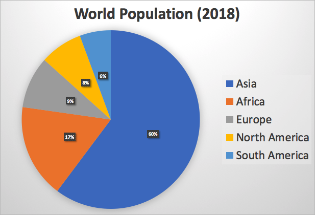
The world population density is ranked similarly (but with South America ahead of North America).
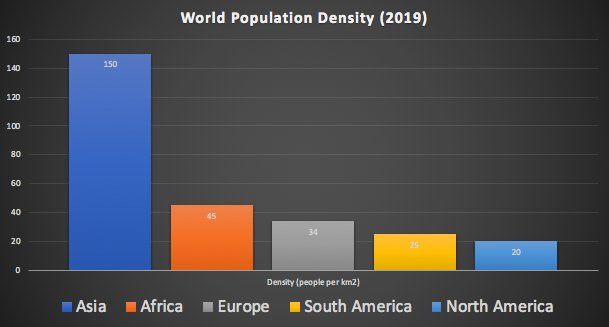
What could this data tell us about placement and resourcing of distributed applications globally? In theory, you need more resources in areas of higher population, and latencies and user experience will be better in areas of higher population density.
However, another map may give a different perspective. Where are potential users most likely to be located based on internet connectivity? This is another cartogram showing the populations of people using the internet (somewhat old 2017 data):
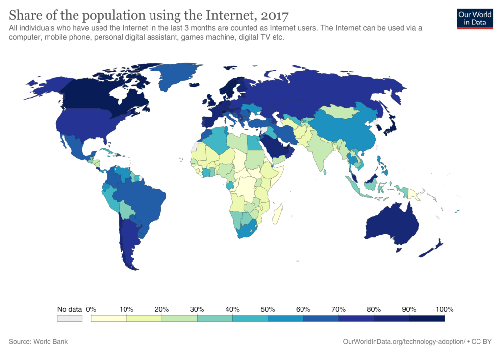
Some observations are that Asia is home to the world’s largest internet population, South America and Africa have sizeable internet populations (300M each, which combined exceeds the European internet population of 550M), and in most of the world’s largest internet countries (i.e. excluding North America, Central Europe, South Korea, Japan) less than 60% of their population is online (so are likely to have growth potential in the future). The growth rate in online users over the last decade has been most in Asia, South America, and Africa. So armed with this background information let’s now take a look at the Public Cloud world.
4. Mapping the Public Cloud
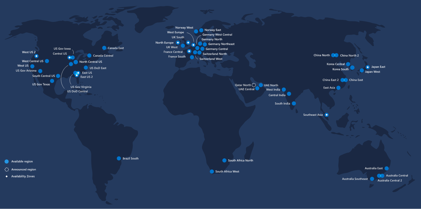
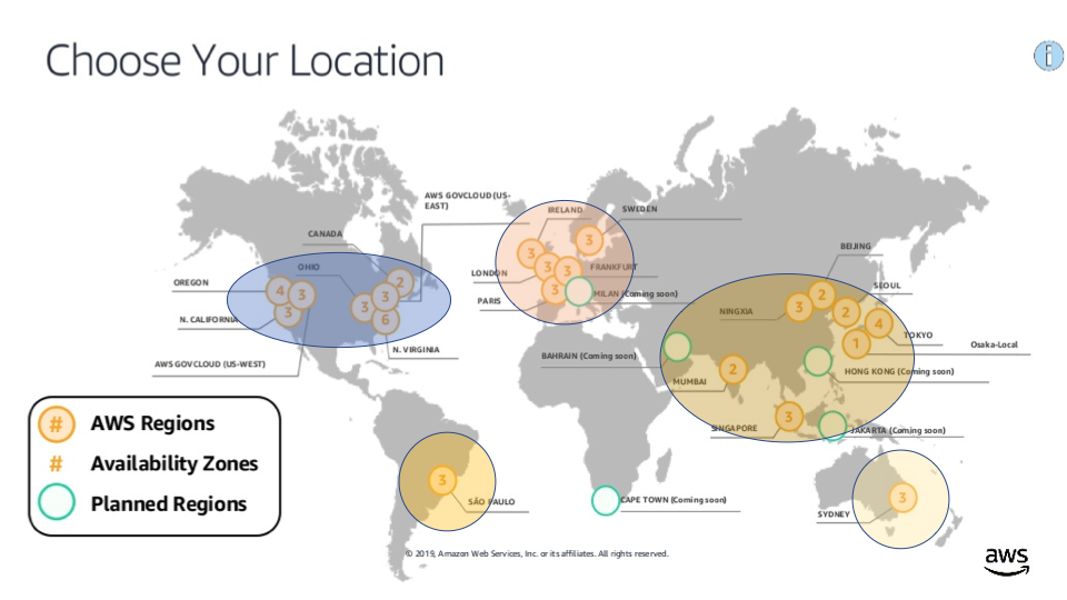
Instaclustr runs managed Open Source Technologies in the 22 AWS regions as follows:
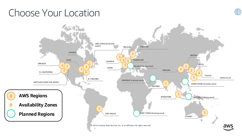
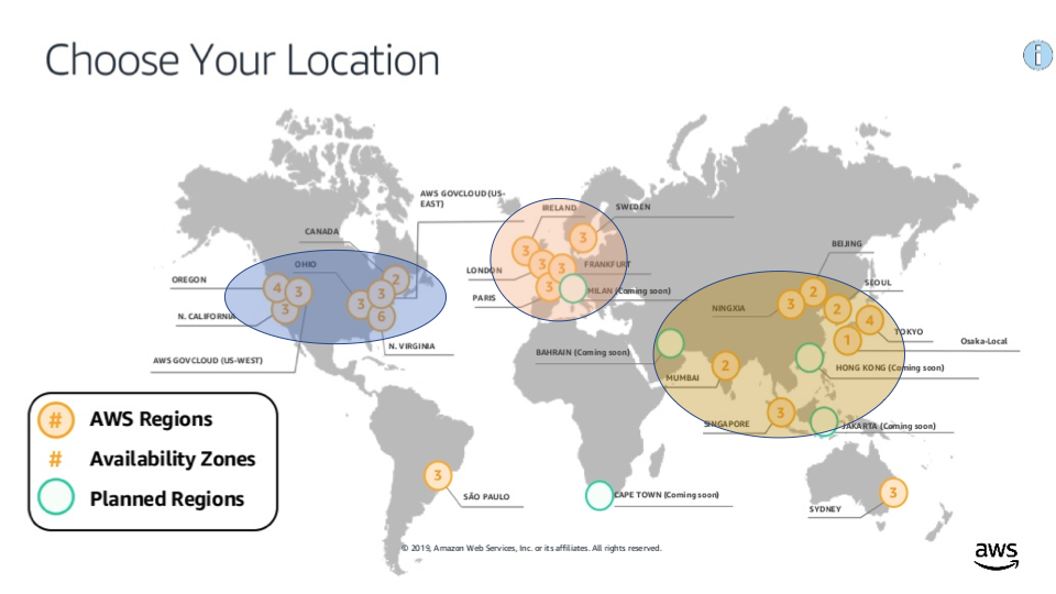
You can also use Google’s Cloud (GCP, 20 regions, with similar locations), or Azure (55 regions, with more choice including Africa, and multiple locations in Australia). There’s a live Azure region map here.
 (Source: build5nines.com)
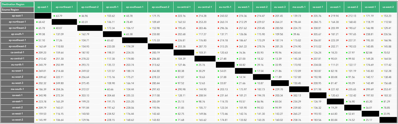
Because they are globally distributed and different distances apart, there is latency between regions. There are a number of 3rd party sites that measure latency between cloud regions including AWS. I used one that measures latency between 18 AWS regions over 24 hour periods (cloudping.co) giving results in a table format like this:
Other tools allow you to measure latency to/from your browser and/or between regions for the major cloud providers (e.g. cloudping.info, gcping.com, and https://cloudpingtest.com/ for multiple clouds). Note that the times from a browser to regions don’t necessarily correspond to cloud inter-region latencies (possibly because of slightly different starting locations, cloud-specific network optimizations). For example, latency from a browser in Canberra (Australia) to the AWS Singapore region is faster than to the AWS Tokyo region, even though AWS Sydney to Tokyo inter-region latency is faster than Sydney to Singapore inter-region latency.
The latency between regions ranged from a minimum of 11ms (London to Paris) to a maximum of 467ms (Bahrain to Sao Paulo) with an average of 163ms. We plotted inter-region latencies on this contour map (a heat map with elevations). Regions that are closer to each other (< 100ms) are shown in dark blue (peaks).
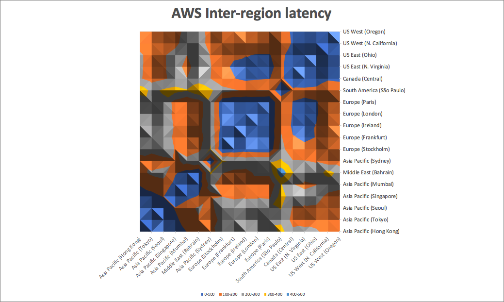
You will notice that some regions are part of big blue “clumps”. The most obvious groupings are North America (including Canada), Europe, and Asia:
The average latency in North America is 55ms, Europe is 26ms, and Asia (excluding Sydney) is 85ms. There are also a couple of outliers, South America, and Sydney, that are not within 100ms latency of any other regions:
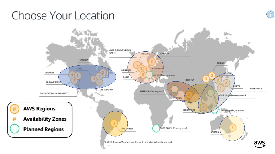
Closer inspection reveals that the Asia clump is actually more spread out than the others, with some regions > 100ms distance from each other (e.g. Tokyo and Bahrain/Mumbai. There are therefore three sub-groupings (with partially overlapping memberships) of AWS regions that are all within 100ms of each other as follows: Bahrain/Mumbai, Mumbai/Singapore/HK, and Singapore/HK/Seoul/Tokyo. Note that as I didn’t have any China region latencies they are not included:
There is also another clump (with overlapping memberships) crossing the Atlantic and including the East Coast of North America and all regions in Europe except Stockholm:
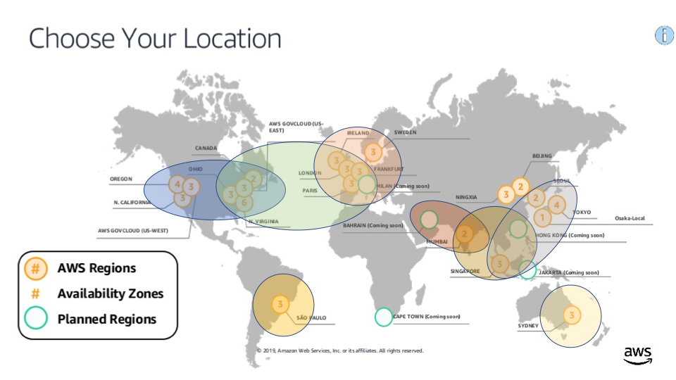
AWS latency clumps (regions within 100ms latency of each other)
5. Around the World: Location
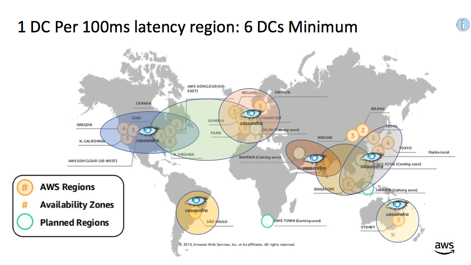
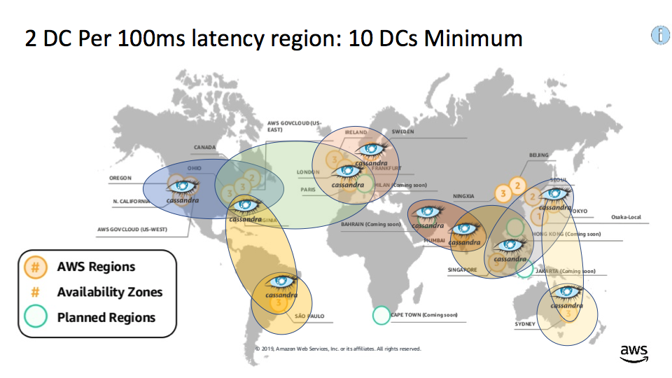
What does this mean in practice? Imagine our goal is to deploy a globally distributed application, with users all around the world, and we want to reduce latency for the users. Where should we deploy the application? To make it more concrete, imagine it’s a Cassandra-based application, with Cassandra clusters and associated Cassandra client and application deployed to one or more regions. We assume we have users in each geographical region (excluding Africa, Alaska and Russia due to lack of data), and a target user to application latency of under 100ms. This means we need a Cassandra cluster and associated application in most of our latency clumps (we use AWS inter-region latencies as a proxy for user to application latencies). A minimum of 6 data centers are required as follows: 1 in North America, 1 in Europe, Sydney, South America, 1 out of Bahrain/Mumbai, 1 out of Singapore/HK/Seoul/Tokyo:
But what if you also want to have multiple data centers for redundancy in each 100ms clump? This is harder to achieve for the 2 outlier regions. However, North Virginia is the closest region to South America (124ms) and Tokyo is the closest to Sydney (109ms), so a possible solution involving a total of 9 data centers could be as follows. The number of data centers in Asia goes up from 2 to 4 due to having 3 (overlapping) clumps to cover redundantly, but the number of DCs in America and Europe only goes from 3 to 4 due to a trick. We use a data center in North Virginia as the backup for 3 clumps, North America, South America, and most of Europe; the rest of Europe (beyond the 100ms latency from the USA East Coast) is covered by an extra data center in Stockholm:

If Transatlantic redundancy and resulting latency (around 100ms) is too high for practical purposes, then another solution using 10 data centers would ensure 2 redundant data centers within Europe as follows (reducing average latency to 26ms within Europe):
Instaclustr sometimes takes a little while to catch up with other new regions for cloud providers (they can be quickly added upon request). We currently offer 12 AWS regions (missing Bahrain and Sweden), so the minimum 8 regions for regional redundancy under 100ms would be: Sao Paulo, North Virginia, Ohio, Ireland, Mumbai, Singapore (which provides close to 100ms latency for Bahrain), Tokyo, Sydney:
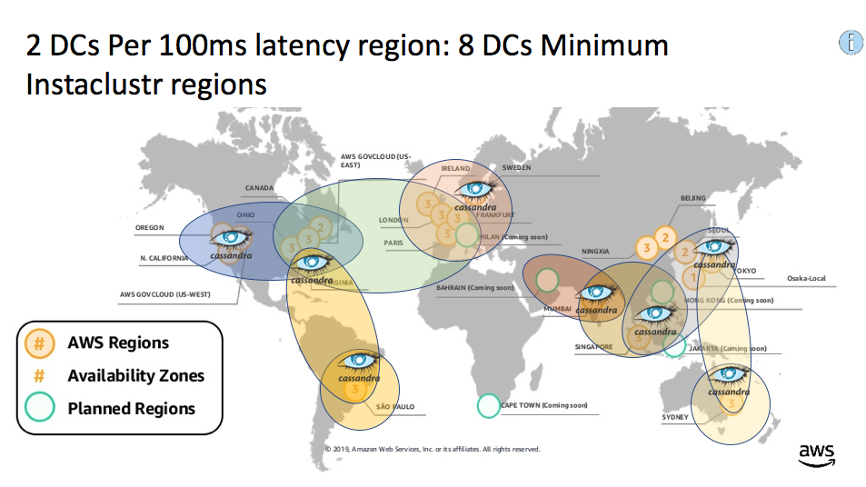
Globally distributed application redundant data centers using Instaclustr available regions
Note that we offer more regions in Azure (15), and GCP (17).
6. What’s Next?
Well, that’s one possible itinerary for our proposed journey “Around the World in (approximately) 8 Data Centers”. As Phileas Fogg quickly discovered, travel plans have to be flexible, so we’ll have to see how well it holds up to the rigours of the actual journey. He also had to use many different modes of transportation. Typical for the era, and the catalyst for the bet was the globally expanding Victorian era railways. But he also had to travel by steamship and even an elephant! Likewise in this blog series, we’ll try out some different technologies for building globally distributed applications. In the next blog we’ll take a closer look at multi-DC/multi-region replication in Apache Cassandra, including how to provision a multi-DC cluster, what topologies/replication patterns are possible, what the replication performance is like, what resources are required due to the replication overhead, will regional clusters be the same size and is this impacted by regional workloads, and what influences the price. Hopefully, the stash of cash in our carpetbag will cover the price of the trip!