Classic lexical search matches tokens: if the user does not use the same words as the document, relevance suffers. Semantic search matches meaning by turning text into embeddings—fixed-length vectors from a neural network—so “car repair” can sit near “automotive service” even when the vocabulary differs. That shift is powerful, but it is not free. You pay in RAM, CPU or GPU for indexing and inference, in latency for ANN (approximate nearest neighbor) search, and in engineering time for tuning hybrid systems that combine lexical precision with semantic recall.
This post is a practical map: how to design indices, shape queries, size clusters, and measure whether the changes you make actually help. OpenSearch evolves quickly; Lucene and Faiss (Facebook AI Similarity Search) differ in how they store vectors, apply filters, and use memory. Treat every recommendation here as a hypothesis—validate on your OpenSearch version, your hardware, and your data. This guide provides practical heuristics and decision frameworks, not prescriptive configurations.
What is AI Search in OpenSearch?
Embeddings are numeric summaries of text (or images, or structured fields) produced by a trained model, often a transformer-based encoder LLM (large language model). Semantically similar inputs should land close together in vector space. At query time you embed the query the same way you embedded the existing data, then retrieve neighbors under a distance or similarity function—commonly cosine similarity, dot product (inner product), or L2 (Euclidean) distance. The metric must match how the model was trained and whether vectors are normalized (e.g., unit length)
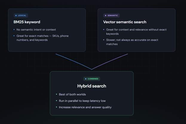
BM25 is a strong lexical ranker: fast, interpretable, excellent for exact tokens (SKUs, error codes, names). OpenSearch k-NN (k-nearest neighbors) over dense vectors captures semantic overlap where keywords diverge. OpenSearch Hybrid retrieval runs both and merges results—because neither alone is ideal for mixed traffic, like natural language queries where key words, titles, or identifiers are common.
Exact k-NN doesn’t scale to large corpora, so many production systems use ANN indexes. HNSW (Hierarchical Navigable Small World) builds a layered proximity graph; IVF (inverted file) partitions the space and searches only a few clusters of vectors in the space (nprobe). You trade a small amount of recall (fraction of true neighbors found) for large gains in speed and resource use.
| kNN (dense vectors) | ANN (sparse vectors) | |
|---|---|---|
| Accuracy | Extremely accurate results | Nearly as accurate as kNN |
| Scale | Does not scale to large document sets and high query volumes | Magnitudes less resource use and lower latency on larger document sets |
In OpenSearch, the pieces you usually wire together are: an index mapping (the schema JSON for an index) with at least one field whose type is rank_features. That field stores each document’s embedding vector and declares how it is indexed for ANN search, including engine (Lucene or Faiss), distance space, graph or IVF method, and build/query parameters.
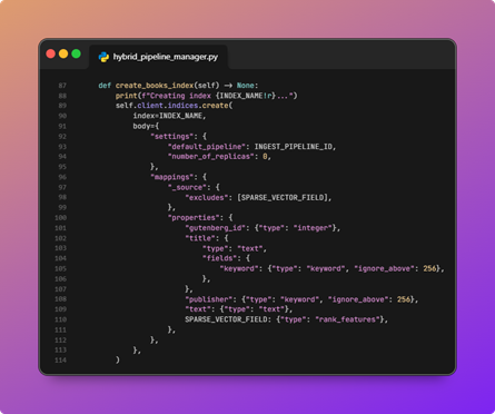
An example of an index mapping with an ingest pipeline and sparse vector features.
Alongside that: ML Commons to host models and run inference; neural search helpers that embed queries and documents; ingest pipelines to compute embeddings as documents are indexed; and search pipelines for score normalization, hybrid combination, and reranking. A useful mental model here, regardless of your stack, is retrieve, rerank, return: cast a wide, cheap net first; apply expensive precision only on a short shortlist.
With that stack and mental model in place, the first place you can make those costs and trade-offs concrete is in index design.
OpenSearch index design for vector search
Pick the embedding model deliberately. One of the largest considerations is dimension (e.g., 384 vs 1024 vs higher), which directly drives resource use and latency cost. Also, check whether the model’s outputs are normalized, and which similarity the model vendor recommends. Consider domain fit and whether to use a large language model or a smaller, more specialized model for things like legal, code, and support tickets. You’ll also want to consider the languages the model supports, and whether you must self-host for compliance. Changing the model usually means re-embedding every single document, so stabilize chunking and metadata first when you can.
Next, configure the vector field to match the workload. The decision that has the most downstream consequences, and the one most people make without realizing it, is Lucene vs Faiss. The documentation presents them as equivalent options with different characteristics. In practice, the fork is meaningful:
- Lucene vector search integrates with the segment lifecycle, applies filters natively during the graph walk so there’s no post-filter result gap, uses OS page cache instead of dedicated off-heap memory, and supports on-disk graph storage for memory-constrained warm tiers.
- Faiss vector search has a wider quantization menu, GPU support, and IVF for very large corpora where HNSW graph overhead becomes the constraint.
For most hybrid text workloads, Lucene is the right default. Reach for Faiss when you have a specific reason. The choice is difficult to change after data is indexed, so be deliberate.
Choose HNSW vs. IVF based on data scale and query pattern:
- HNSW is the default mental model for many text workloads
- IVF can win at very large scale with careful tuning
- Set
m(graph connectivity) andef_construction(build quality) such that you can tuneef_searchat query time against your recall–latency curve
Also, consider quantization, which can shrink the memory and storage footprint of vectors significantly:
- FP32 (32-bit floating point) is the baseline way vectors are stored
- FP16 (16-bit floating point) saves nearly half the space with often modest recall impact
- Byte / scalar quantization goes further to 8-bit integers, and PQ (product quantization) compresses aggressively for huge corpora at higher recall risk
Use recall@k and precision@k to measure how aggressively you want to quantize and save resource use over recall.
Design for hybrid from day one. Store text, structured filters, and vectors on the same logical documents so one request can combine BM25, k-NN, and filters. Use keyword, numeric ranges, and dates for filters the ANN layer can exploit to shrink the candidate set before expensive model computation (pre-filtering).
Size shards so each shard holds a manageable vector set for your QPS (queries per second) target; add replicas for read scaling and availability, knowing each replica multiplies storage and memory.
OpenSearch hybrid search query strategy
It is recommended to keep a BM25 search as a part of your query. It’s cheap to run in parallel with semantic searches and often wins on exact matches.
For OpenSearch k-NN search, k (how many neighbors you ask for) and ef_search (how hard HNSW searches) are the main levers you can pull at search time. Raising them improves recall but pushes p95/p99 (95th/99th percentile) latency. Plot recall vs latency when testing, instead of tuning your settings by gut feel.
Hybrid search needs comparable score scales. Search pipelines can normalize lexical and vector scores—for example min–max scaling, or L2 normalization applied to a vector of subscores (rescaling the tuple of BM25 and vector contributions to unit length). That’s not the same thing as L2 distance between document embeddings in vector space, which is a retrieval metric, not a hybrid score-combination step.
Alternatively, use RRF (reciprocal rank fusion), which merges ranked lists from each subquery using rank positions instead of raw scores—often more stable when score distributions differ wildly. Tune weights or RRF parameters on an offline eval set, not on a handful of hand queries.
Filtered k-NN is where production surprises hide. Pre-filtering applies filters before the graph walk, which is accurate but can leave too few candidates. Post-filtering is fast but may return empty or tiny result sets if neighbors fail the filter. Prefer engine paths that apply filters efficiently when available, and measure recall under realistic filter selectivity, not only on unfiltered dev data.
Reranking is the precision layer. A cross-encoder (or similar) scores query–document pairs jointly and beats bi-encoder similarity, but at much higher cost per document. Use ML Commons (or an external service) to rerank only the top-N from retrieval; N is your primary latency dial. For RAG (retrieval-augmented generation), align chunk boundaries with how answers appear in text, deduplicate near-identical chunks, and return enough context for the downstream LLM without flooding its context window and diluting signal.
Resource and cluster tuning for managed OpenSearch
Memory planning starts from vector_count × dimensions × bytes_per_value plus ANN index overhead (for HNSW, overhead grows with m). Faiss often relies on native, off-heap memory; Lucene leans on memory-mapped segments and the OS page cache. Undersized RAM shows up as churn, GC (garbage collection) pressure on the JVM, or cold-cache latency spikes, not just “slow queries.”
| Question | If yes | If no |
|---|---|---|
| Working set fits in RAM (per replica on node)? | Memory-optimized hot tier | Quantize / split / tier / accept miss latency |
| HNSW m high for recall? | Budget extra RAM | Lower m or accept recall loss |
| Replicas on same node? | Multiply RAM need | Spread replicas across nodes |
Heap vs off-heap: Oversized JVM heaps steal RAM from Faiss graphs and from the OS cache backing Lucene. Follow OpenSearch guidance for your distribution; vector-heavy clusters usually want a moderate heap and plenty of non-heap RAM for graphs and caching.
| Symptom | Action |
|---|---|
| Good knn but GC pauses on aggs | Slightly increase heap within guidance |
| knn slow, high disk read, modest GC | Decrease heap; add RAM to node for cache/native |
| Faiss OOM / RSS at limit | Increase node RAM or reduce graph size; don’t only grow heap |
Hardware and tiers: Prefer memory-optimized nodes for hot vector indices; use fast NVMe (Non-Volatile Memory express) or SSD (solid-state drive) storage for warm data; push cold or rarely queried data to cheaper tiers or searchable snapshots when latency SLOs (service-level objectives) allow.
| Query pattern | Tier |
|---|---|
| knn on every request, tight p99 | Hot: RAM + NVMe |
| Daily analytics, loose p99 | Warm: SSD |
| Rare legal / archive search | Cold: searchable snapshot / cheap storage |
Concurrency and segment hygiene: Watch search and knn thread pools and queue rejections under load. Warm caches after deploys and major merges—cold ANN graphs hurt tail latency. A lower refresh_interval improves search freshness but creates more segments and merge work; force-merge can help read-only indices but is operational baggage on active writes—balance segment count, ingest rate, and tail latency.
| Situation | Settings to change: |
|---|---|
| Real-time ingest, freshness SLO | Lower refresh_interval + accept merge cost |
| Stable index, tail latency SLO | Higher refresh_interval + fewer segments |
| Rolled, read-only index | forcemerge in maintenance window + warm-up |
| Active writes | No forcemerge; tune refresh + merge |
Measuring quality, latency, and cost in OpenSearch
Offline evaluation grounds decisions. Build a set of queries with graded relevance judgments (or carefully audited LLM labels). Report:
Recall@k(whether the right doc appears in the top k)- nDCG (normalized discounted cumulative gain): Quality-aware ranking)
- MRR (mean reciprocal rank): Where the first relevant hit sits.
Track these metrics whenever you change embeddings, ANN parameters, hybrid weights, or rerankers.
Online, split metrics by path taken: keyword-only, pure k-NN, hybrid, reranker should all be separately delineated steps. Report and track on p50/p95/p99 latency, QPS, error rates, and queue rejections to detect problems before they take down your cluster. A change that flatters p50 but hurts p99 is often a production incident in disguise.
Cost belongs in the same dashboard: approximate dollars per million queries, RAM per million vectors, and ingest cost per document (embedding dominates many pipelines). Use OpenSearch Dashboards, Search Relevance Workbench where available, and A/B (split) tests on a slice of traffic when you can.
Process beats heroics: Baseline, change one knob, re-run offline metrics and tail latency, then keep or revert. Without that loop, “we made search smarter” usually means “we shifted the failure mode.”
Getting started with managed OpenSearch
AI search in OpenSearch is not a single switch—it is index design, query strategy, cluster sizing, and measurement working together. Engines and features change; NMSLIB is legacy, Lucene and Faiss are the path forward.
Pick one bottleneck this week, whether that’s recall at a fixed p95, RAM per million vectors, or hybrid weights on a frozen eval set. Measure it, change one thing, and iterate. That habit turns OpenSearch vector search from a demo into a system you can run for years.
Ready to put this into practice? Start your own demo OpenSearch cluster with the Instaclustr free trial.
Frequently Asked Questions
-
What is AI search in OpenSearch? +
AI search in OpenSearch uses embeddings—numeric representations of text or data—to enable semantic search. It retrieves results based on meaning rather than exact keywords, offering more relevant search outcomes for complex queries.
-
What is the difference between k-NN and ANN in OpenSearch? +
k-NN (k-nearest neighbor) provides highly accurate search results but struggles to scale for large datasets. ANN (approximate nearest neighbor) trades slight accuracy loss for faster performance and reduced resource usage, making it ideal for large-scale systems.
-
How can I improve hybrid search performance in OpenSearch? +
To optimize hybrid search, combine BM25 for exact matches with vector-based k-NN for semantic relevance. Tune query parameters, normalize score scales, and use efficient pre-filtering to balance recall, latency, and resource usage.