“The thing’s hollow — it goes on forever — and — oh my God! — it’s full of stars!”

It’s full of Spreadsheets! (DataFrames)

(Source: Wikimedia Commons)

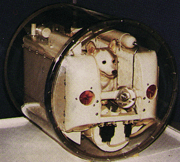
Given that a dog, Laika, was the 1st astronaut to orbit the earth, it’s appropriate for a dog to travel through the wormhole.

After travelling through the wormhole, the 2001 story (book version, as is the “it’s full of stars” quote which is not in the movie) concludes.

Dave leaves the pod and explores the hotel room. He finds a telephone and telephone book, but the phone doesn’t work and the telephone book is blank. He explores more and finds a refrigerator, where there is a variety of packaged food, but it all contains the same blue substance (even, to his disappointment, in the beer cans). He eats the blue food, and drinks the tap water—which tasted terrible—because, being distilled water, it had no taste at all. He turns on a television but all the programs were two years old. Dave lies down on the bed, turns off the light and “So, for the last time, David Bowman slept.”

(Source: Wikimedia Commons)

What’s new in this blog? DataFrames (giant Spreadsheets), ML Pipelines and Scala!

As I noted last blog, the trip took a while and the TV shows are old. The ML API for Spark is now based on the DataFrame API:

https://spark.apache.org/docs/latest/ml-guide.html

The MLlib RDD-based API is now in maintenance mode.

As of Spark 2.0, the RDD-based APIs in the spark.mllib package has entered maintenance mode. The primary Machine Learning API for Spark is now the DataFrame-based API in the spark.ml package.

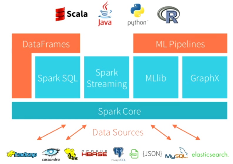
This architecture diagram shows the current Spark architecture. The components of particular interest are Cassandra (the data source), MLlib, DataFrames, ML Pipelines and Scala:

Last blog we explored Decision Tree Machine Learning based on RDDs, using a sample of the Instametrics monitoring data, to try and predict long JVM Garbage Collections. Now we’ll update the code to DataFrames and use all the available real monitoring data (a snapshot from the Instaclustr pre-production clusters).

What are DataFrames? Big, distributed, scalable spreadsheets! They are immutable and can be transformed with a DSL, pre-defined functions, and user-defined functions.  

Scala Code

Why did I ditch Java (at least temporarily)? Have I become “transcendent” after watching 2001 too many times?

Not exactly. Because Instaclustr provides a fully managed cluster option which includes Cassandra, Spark, and Zeppelin (a Spark Scala web-based notebook) it was easier to quickly deploy, run and debug Scala code than Java. You just type Scala code into Zeppelin in a browser, run it and look at the output (and repeat). There’s no need to set up a separate client instance in AWS. Trying to learn both Scala and Spark at the same time was “fun”. Scala is syntactically similar to Java (just throw away the semi-colons as Scala is line-oriented, and you don’t need variable type declarations as types are inferred, but statically typed), so the example should still make sense even without any Scala experience (like me).

For example:

var anyGreeting = “Hello world!” // universal greeting
val queenGreeting = “How do you do?” // How to greet the Queen (of England)

// equivalent to
var anyGreeting : String = “Hello world!”
val queenGreeting : String = “How do you do?”

vars are mutable and can be changed, vals are immutable and can’t be changed, so:

anyGreeting = “Kia ora” // hello in Maori
queenGreeting = “Ow ya goin mate” // hello in Australian, won’t work as immutable
anyGreeting = 3.14159 // won’t work, as anyGreeting is a String

Let’s revisit the Decision Tree ML code in Scala + DataFrames.

Here’s the latest documentation for the Decision Tree Classifier for DataFrames.

As the Instametrics monitoring data we have is in Cassandra we need to read the data into Spark from Cassandra first. To do this we use the Spark Cassandra connector.

Instaclustr provides a Spark Cassandra assembly Jar.

In Zeppelin (more on Zeppelin in a future blog) this is loaded as follows:

Then lots of imports (in Zeppelin you have to run each line separately):

In Zeppelin, the spark context will already be defined for you, and there are helper functions to simplify reading in a Cassandra table. For some reason, the 1st argument to cassandraFormat is the table name, and the 2nd is the keyspace.  This returns (lazily) a DataFrame object.

val data = spark
.read
.cassandraFormat(“mllib_wide”, “instametrics”)
.load()

Loading lots of data from Cassandra works well, it’s fast, and DataFrames infers the schema correctly.  The format of the data DataFrame is lots of examples (Rows) with columns as follows (wide table format has each data variable/feature in a separate column):

<host, bucket_time, label, metric1, metric2, metric3, …>

Where did this data come from? From some complex pre-processing (next blog). The label column was also previously computed and saved (the label is the class to be learned, in this case either 1.0 for positive examples, or 0.0 for negative examples).

The next trick is to replace null values with something else (e.g. 0), as we run into problems with nulls later on (even though in theory the MLLib algorithms cope with sparse vectors).

val data2 = data.na.fill(0)

Here are the relevant documents:

https://spark.apache.org/docs/1.3.1/api/scala/index.html#org.apache.spark.sql.DataFrame

https://spark.apache.org/docs/1.4.0/api/java/org/apache/spark/sql/DataFrameNaFunctions.html

As in the previous RDD example we need two subsets of the data, for training and testing:

val Array(trainingData, testData) = data2.randomSplit(Array(0.7, 0.3))

Next we need to produce an Array(String) of column names to be used as features. In theory all of the columns can be used as features, except the label column, but in practice some columns are not the correct type for the classifier and must be filtered out (e.g. for this example we can only have Doubles):

val featureCols = data2.columns.filter(!_.equals(“host”)).filter(!_.equals(“bucket_time”)).filter(!_.equals(“label”))

Next we need to create a single column of features. VectorAssembler is a transformer that combines a list of columns into a single vector column, which is what we want.  However, it turns out to have problems with null values (which is why we replaced them above).  

val features = new VectorAssembler()
.setInputCols(featureCols)
.setOutputCol(“features”)

Here’s the VectorAssembler documentation:

https://spark.apache.org/docs/2.1.0/ml-features.html#vectorassembler

https://spark.apache.org/docs/2.1.0/api/scala/index.html#org.apache.spark.ml.feature.VectorAssembler

Next create a DecisionTreeClassifier, with the column to predict as “label”, and the features to use called “features” (from the VectorAssembler above):

val dt = new DecisionTreeClassifier()
.setLabelCol(“label”)
.setFeaturesCol(“features”)

More documentation:

https://spark.apache.org/docs/1.5.2/ml-decision-tree.html

https://spark.apache.org/docs/2.0.0/api/java/org/apache/spark/ml/classification/DecisionTreeClassifier.html

Pipelines, Tunnels, Wormholes

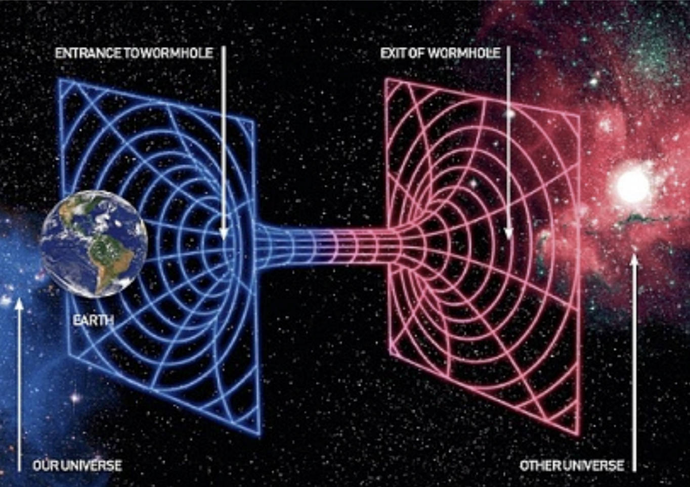
Another new Spark feature is Pipelines (tunnels, wormholes, etc).  A Pipeline chains multiple Transformers and Estimators together for a ML workflow. A Transformer is an algorithm (feature transformers or learned models) that can transform one DataFrame into another DataFrame (e.g. a ML model transforms a DataFrame with labels and features into a DataFrame with predictions). An Estimator is an algorithm that can be fit on a DataFrame to produce a Model (which is a Transformer). This Pipeline consists of only two stages, features (feature transformer) and dt (estimator) (More on stages):

val pipeline = new Pipeline()
.setStages(Array(features, dt))

Now we actually train the model by calling the pipeline fit method on the trainingData:

val model = pipeline.fit(trainingData)

And then test it by applying the model to the testData. This produces a DataFrame with a “predictions” column (by default), a “label” column (actual class), and the “features” column:

val predictions = model.transform(testData)
predictions.select(“prediction”, “label”, “features”)

 The MulticlassClassificationEvaluator can compute a limited number of evaluation metrics, here’s an example for “accuracy”:

val evaluator = new MulticlassClassificationEvaluator()
        .setLabelCol(“label”)
.setPredictionCol(“prediction”)
.setMetricName(“accuracy”)

val accuracy = evaluator.evaluate(predictions)
println(“Test Error = ” + (1.0 – accuracy))

However,  as pointed out the previous blog the model accuracy isn’t a particularly useful metric depending on the actual ratio of positive/negative examples.  We can use the MulticlassMetrics to compute the confusion matrix, precision, and recall. And then also compute the actual rate of negative examples for comparison with the model accuracy metric. MulticlassMetrics has an auxiliary constructor for DataFrames but I still had to convert to an RDD before use. See this book for more information and ways of creating a confusion matrix from a DataFrame directly.

And now print the model out.

val treeModel = model.stages(1).asInstanceOf[DecisionTreeClassificationModel]
println(“Learned classification tree model:\n” + treeModel.toDebugString)

The decision tree actually doesn’t make much “sense” as the named features have been replaced by feature numbers (e.g. If (feature 23 <= 8720.749999999996) Predict 0.0 Else etc). Ideally there should be some way of automatically converting them back to the original names.

Results

Did it work? I’m sorry, I can’t tell you. In theory after going through the wormhole, information flow to the outside world is limited (the telephone didn’t work).  Ok, we’re not really in some virtual reality hotel/zoo at the other end of the universe (probably), and Dave did travel back to this universe, so I can tell you…

For this example we used real data, but obtained from our pre-production clusters. Rather than pre-process all the raw data I took a shortcut and use the rolled up data which had min, avg and max values computed for every metric over 5 minute periods. However, I forgot to check the bucket_time values, and later discovered that the bucket_time was actually hourly, so I ended up using hours as the default time period for learning. I also noticed that the JVM GC durations had not been rolled up for this snapshot of data, so I used these read and write SLA metrics to compute the label:

/cassandra/sla/latency/read_avg(avg)
/cassandra/sla/latency/read_max(max)
/cassandra/sla/latency/write_avg(avg)
/cassandra/sla/latency/write_max(max)

These metrics were combined with thresholds to ensure that about 5% of the examples were positive (i.e. had “long” read/write times). And these metrics were removed from the data before use to prevent cheating by the machine learning algorithm.

The wide data table read from Cassandra had 1518 examples (rows), which was split into training and test data. The training data set had 1067 examples, but only 60 positive examples (not a huge number for a Big Data problem, and in practice the number of examples needs to be >> the number of features, at least 2x). There were 2839 features (columns).

Learning only took a few minutes. Model accuracy was 0.96, however, as the negative example rate was 0.95 this isn’t much better than guessing. Precision was 0.60 and Recall was 0.66.

Is this result any good? A precision of 0.6 means that given a prediction of a SLA violation by the model, it is likely to be correct 60% of the time (but gets it wrong 40% of the time). A recall of 0.66 means that given an actual SLA violation, the model will correctly predict it 66% of the time (i.e. but misses it 34% of the time).  By comparison, using a sample of the data in the previous blog the recall was only 45%, so 66% is an improvement! Assuming that the cost of checking a SLA violation warning (from the model prediction) is minimal, then it’s more important to correctly predict as many actual SLA violations (assuming we can do something to prevent/mitigate them in advance, and that SLA violations are expensive if they occur), and increase the recall accuracy.   How could this be done? More and better quality data (e.g. from production clusters, as pre-production clusters and metrics are somewhat atypical, for example, many nodes may be spun up and down for short time periods, and they don’t have typical user workloads running on them), reducing the number of features (e.g. feature selection, by removing redundant or highly correlated features), and different ML algorithms…

What features did the model pick to use to predict the long SLAs times from the 2839 features available? Only these 11 (which appear to be plausible):

1. /cassandra/jvm/memory/heapMemoryUsage/max
2. /cassandra/jvm/memory/heapMemoryUsage/used_avg
3. /cassandra/metrics/type=ClientRequest/scope=Read/name=Latency/95thPercentile_avg
4. /cassandra/metrics/type=ClientRequest/scope=Read/name=Latency/count_max
5. /cassandra/metrics/type=ClientRequest/scope=Read/name=Latency/latency_per_operation_avg
6. /cassandra/metrics/type=ClientRequest/scope=Write/name=Latency/95thPercentile_avg
7. /cassandra/metrics/type=ClientRequest/scope=Write/name=Latency/latency_per_operation_avg
8. /cassandra/metrics/type=ColumnFamily/keyspace=test/scope=testuncompressed/name=TotalDiskSpaceUsed_max
9. /proc/diskstats/xvda1/sectorsWritten_max
10. /proc/diskstats/xvdx/sectorsRead_avg
11. /proc/stat/cpu-agg/user_max

Thanks to Instaclustr people for help (with Instametrics data, support for Cassandra, Spark and Zeppelin, and machine learning discussions) including Christophe, Jordan, Alwyn, Alex_I, Juan, Joe & Jen.

Next Blog

How did we get here? Next blog we’ll look behind the scenes at the code that was used to preprocess the raw metrics from Cassandra, clean the data, convert it into the wide table format, and correctly label the examples. And, how to run Spark Scala code in Zeppelin!

(Source: Shutterstock)

Instaclustr SPARK Trial Offer

You can try out a special offer of an Instaclustr trial cluster provisioned with Cassandra, Spark, and Zepplin using the coupon code ST2M14:

https://console.instaclustr.com/user/signup?coupon-code=ST2M14

CODE

Next Blog: Behind the Scenes