Third contact with a Monolith: Sensor Scan

Apache Cassandra
Technical

Third contact with a Monolith—Long Range Sensor Scan

September 14, 2017
By Instaclustr

Distance of the Planets from the sun in Astronomical Units Instaclustr

The Odyssey Continues: A Long Trip to Jupiter

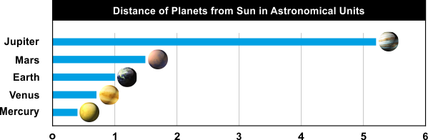
Earth to Mars distance = 0.52 AU (1.52-1AU, 78M km)

Earth to Jupiter distance = 4.2 AU (5.2-1AU, 628M km)

It’s a long way to Jupiter, would you like to:

(a) sleep the whole way in suspended animation? (bad choice, you don’t wake up)

(b) be embodied as HAL the AI? (go crazy and get unplugged)?

(c) be one of the two crew to stay awake the entire journey (only one of you survives)?

What can we do to find out more about our eventual destination the meantime and relieve the boredom?

In the traditions of the best sci-fi, there are always tricks to speed things up or cut down on the special effects budget. In Star Trek these were Sensors to Scan distant phenomenon. And the Transporter which used Materialization and Dematerialization to beam people to and from the ship and the surface of planets.

Energize!

(Source: Wikimedia Commons)

At the risk of mixing sci-fi movie metaphors:

“Captain’s Log, Stardate 1672.1. Warp drive offline. We’re running on auxiliary impulse engines to Jupiter to explore an anomaly. Our mission is to explore a snapshot of the Instametrics monitoring data on a Cassandra cluster that has appeared around the orbit of Jupiter. Our goal is to predict long JVM garbage collection durations at least five minutes in advance. Initiating long-range sensor scans after which I will attempt a risky long-range transportation down to the surface of the anomaly.”

Let’s get Cassandra to do all the hard work to reduce the amount of data we need to transfer from the cluster to my laptop. There are two approaches that may result in some useful insights. Calculating some summary statistics, and creating a materialized view.

The first challenge is connecting to the Cassandra cluster. Unlike the trial cluster example I used previously, this cluster had been created with private IP broadcast_rpc_adresses rather than public IP addresses. Does this mean I can’t connect to the cluster from outside the private address range at all? Not exactly. You can still connect via a single public IP address, which will then become the only controller node your client communicates with. For testing, this is probably ok, but there is a better solution using VPC peering and the private IP addresses.

The next step is to see what JVM GC related metrics were collected.

Connecting via the cqlshell, we can run some CQL commands.

Describe instametrics;

Reveals that there are some meta-data tables which contain all the host names, and all the metric (“service”) names for each host:

CREATE TABLE instametrics.host (
    host text PRIMARY KEYwas
)

CREATE TABLE instametrics.service_per_host (
    host text,
    service text,
    PRIMARY KEY (host, service)
) WITH CLUSTERING ORDER BY (service ASC)

CREATE TABLE instametrics.host (

host text PRIMARY KEYwas

)

CREATE TABLE instametrics.service_per_host (

host text,

service text,

PRIMARY KEY (host, service)

) WITH CLUSTERING ORDER BY (service ASC)

How many nodes are there in this sample data set?

cqlsh> select count(host) from instametrics.host;

system.count(host)
————————–
591

The next question I had was how many metrics are there per node? Using a sample of the host names found in the host table I ran this query a few times:

select count(service) from instametrics.service_per_host where host=’random host name’;

The somewhat surprising answer was between 1 and lots (16122!). About 1000 seemed an average so this means about 591*1000 metrics in total = 591,000.

From this distance, we therefore need to focus on just a few metrics. Selecting all the metrics available for one host we find that the following are the only metrics directly related to JVM GC.

collectionCount is the count of the GC, and collectionTime is the total GC collection time, since last JVM restart.

/cassandra/jvm/gc/ConcurrentMarkSweep/collectionCount

/cassandra/jvm/gc/ConcurrentMarkSweep/collectionTime

duration is the time of the last occurring GC, and startTime and endTime are the time of the start and end of the last occurring GC.

/cassandra/jvm/gc/ConcurrentMarkSweep/lastGc/duration

/cassandra/jvm/gc/ConcurrentMarkSweep/lastGc/endTime

/cassandra/jvm/gc/ConcurrentMarkSweep/lastGc/startTime

I normally start a data analysis by looking at statistics for some of the metrics of interest, such as distribution (e.g. a CDF graph) or a histogram. But to compute these statistics you need access to all the data…

Buckets

Kirk: “Mister Spock. Full sensor scan of the anomaly, please.”

Spock: “Captain, the results are not logical – I’m picking up what looks like Buckets – Fascinating!”

Buckets can be problematic:

A drop in the bucket
To kick the bucket
There’s a hole in my bucket

The table with the actual values for the hosts and services is defined as follows:

CREATE TABLE instametrics.events_raw_5m (
    host text,
    bucket_time timestamp,
    service text,
    time timestamp,
    metric double,
    state text,
    PRIMARY KEY ((host, bucket_time, service), time)
) WITH CLUSTERING ORDER BY (time DESC)

CREATE TABLE instametrics.events_raw_5m (

host text,

bucket_time timestamp,

service text,

time timestamp,

metric double,

state text,

PRIMARY KEY ((host, bucket_time, service), time)

) WITH CLUSTERING ORDER BY (time DESC)

The partition key requires values for host, bucket_time and service to select a subset of rows. What’s bucket_time? Based on the name of the table and inspecting a sample of the rows, it’s the timestamp truncated to 5 minute bucket periods. How do we find the range of bucket_time values for the table? Here’s a few ways… You just “know it” (but I don’t). The range has been recorded in another table (not that I can see). Or, start from now and search backwards in time by 5 minute intervals. This assumes that the data is really from the past and not the future. Start from the Epoch and search forward? Do a binary search between the Epoch and now? Look at samples of the data? This revealed that at least some of the data was from the early part of 2016. This would give us a starting point to search forwards and backwards in time until gaps are detected when we can assume they are the temporal boundaries of the data (assuming there aren’t large gaps in the data).

An alternative approach is to make a copy of the table with bucket_time removed from the partition key. Is this possible? Well, yes, in theory. Materialized VIews are possible in Cassandra, and can even be created from existing tables. I created two materialized views, one with the values ordered (descending), and one with the time ordered (ascending).

Create materialized view instametrics.host_service_value as
	Select metric
	From instametrics.events_raw_5m
	Where host is not null and service is not null and metric is not null and bucket_time is not null and time is not null
	PRIMARY KEY((host, service), metric, bucket_time, time)
with clustering order by (metric desc);

Create materialized view instametrics.host_service_time as
	Select metric
	From instametrics.events_raw_5m
	Where host is not null and service is not null and metric is not null and bucket_time is not null and time is not null
	PRIMARY KEY((host, service), time, bucket_time)
with clustering order by (metric asc);

Create materialized view instametrics.host_service_value as

Select metric

From instametrics.events_raw_5m

Where host is not null and service is not null and metric is not null and bucket_time is not null and time is not null

PRIMARY KEY((host, service), metric, bucket_time, time)

with clustering order by (metric desc);

Create materialized view instametrics.host_service_time as

Select metric

From instametrics.events_raw_5m

Where host is not null and service is not null and metric is not null and bucket_time is not null and time is not null

PRIMARY KEY((host, service), time, bucket_time)

with clustering order by (metric asc);

Note that the rules for Materialized Views are very specific. You have to include all the columns from the original PRIMARY KEY in the new table (but they can be in the partition or cluster keys and in different orders), you can include at most one extra column in the new primary key, and the select has to be present and include at least one column – even though the partition key columns are selected by default). The idea was to use the first materialized view to get some summary statistics of the GC durations (e.g. min, average, max), and the second for queries over specific time periods and metrics (to find GCs, and heap memory used between GCs).

This worked as expected, taking 172 seconds, with these results:

Total time = 172343, nodes = 591

Overall stats: Min = 47.0

Overall stats: Avg = 6555.39

Overall stats: Max = 56095.0

The maximum GC duration was 56s, with an “average” of 6.5s.

Here’s the partial code I used:

On closer inspection, the average values were incorrect, as the GC duration values are repeated for multiple timestamps. However, I also obtained the max GC duration for each node, revealing that about 200 nodes (out of 591) had maximum GC durations greater than 10s. This is a good start for “remote” data analysis.