This blog provides an exploration of Spark Structured Streaming with DataFrames
The blog extends the previous Spark MLLib Instametrics data prediction blog example to make predictions from streaming data. We demonstrate a 2-phase approach to debugging, starting with static DataFrames first, and then turning on streaming. Finally, we explain Spark structured streaming in more detail by looking at the trigger, sliding, and window time.
Stream:
/striːm/
A small continuously flowing watercourse.
Creek:
/kriːk/
(Australia) an ephemeral stream, often dry, but occasionally floods.
The Australian Outback can be extreme (hot, dry, wet).
Many roads have restrictions!
 (Source: Shutterstock)
River:
/ˈrɪvə/
(Australia) see Creek.
The Todd River Race is a “boat” race held annually in the dry sandy bed of the Todd River in Alice Springs, Australia (although it was canceled one year—due to rain!)

(Source: Alli Polin – Flickr: Boat Race in the Desert, CC BY-SA 2.0, https://commons.wikimedia.org/w/index.php?curid=25241465)
Apache Spark supports Streaming Data Analytics. The original RDD version was based on micro-batching. Traditionally “pure” stream processing works by executing the operations every time a new event arrives. This ensures fast latency but it is harder to ensure fault tolerance and scalability. Micro-batches were a trade-off and worked by grouping multiple individual records into batches for processing together. Latencies of around 2 seconds were realistic, which was adequate for many applications where the timescale of the trends being monitored and managed is longer than the latency of the micro-batches (i.e. > 2s). However, in practice, the batching latency is only one contributor of many to the overall latency of the system (not necessarily even the main contributor).
The current “Spark Structured Streaming” version supports DataFrames, and models stream as infinite tables rather than discrete collections of data. The benefits of the newer approach are:
- A simpler programming model (in theory you can develop, test, and debug code with DataFrames, and then switch to streaming data later after it’s working correctly on static data); and
- The time model is easier to understand and may have less latency.
1. Dry Run: DataFrame Design and Debugging
The Todd River is dry for most of the time!

(Source: Shutterstock)
The streaming problem we’re going to tackle in this blog is built on the predictive data analytics exploration in the previous blogs. Let’s say we have produced a model using Spark MLlib which can be applied to data over a time period (say 10 minutes) to predict if the SLA will be violated in the next 10 minute period and we want to put it into production using streaming data as the input. Rather than dividing the streaming data up into fixed 10-minute intervals, forcing us to wait for up to 10 minutes before obtaining an SLA warning, a better approach is to use a sliding window (e.g. 1-minute duration) that continuously updates the data available and aggregation calculations (such as a moving average) every minute. This will ensure that we get SLA warnings every minute – i.e. every minute (sliding interval) we want to know what happened over the last 10 minutes (window duration).
After spending several frustrating days attempting to design, debug and test a complete solution to a sample problem involving DataFrames and Spark Streaming at the same time, I recommend developing streaming code in two steps. First (1) design and debug a static DataFrame version, and then (2) add streaming. In theory, this should work as you can focus on the correct series of DataFrame transformations required to get from your input data to the desired output data, and then test it with static data. Also given that Spark DataFrames use lazy evaluation it’s best (for sanity) to test each operation in order before combining them. All without having to also worry about streaming data issues (yet).
Here’s the initial pure DataFrame code (I developed and ran this code on an Instaclustr Spark + Zeppelin cluster, see last blog on Apache Zeppelin):
|
1 2 3 4 5 6 7 8 9 10 11 12 13 14 15 16 17 18 |
val windowDuration = "10 minutes" // how much data to retain in window val slideDuration = "1 minutes" // how often to update the data case class Raw(node: String, service: String, metric: Double) val inSeq = Seq(Raw("n1", "s1", 1.0), Raw("n1", "s1", 10.0), Raw("n1", "s2", 2.0), Raw("n2", "s1", 33.0)) val inDF = inSeq.toDF() val outSLA = inDF .withColumn("time", current_timestamp()) .filter($"service" === "s1" || $"service" === "s2") .withColumn("window", window($"time", windowDuration, slideDuration)) .groupBy("node", "window") .pivot("service") .agg(min("metric"), avg("metric"), max("metric")) .filter($"s1_avg(metric)" > 3 && $"s2_max(metric)" > 1) .select("node", "window") |
The variables windowDuration and slideDuration are Strings defining the window size and sliding window times. Next, we define a class Raw and Seq inSeq (a few samples) for the raw data (with node, service, and metric fields). This uses the scale “case class” syntax which enables automatic construction. We then turn the inSeq data into a DataFrame (inDF).
To this raw data DataFrame, we apply a series of dataFrame transformations to turn the raw input data into a prediction of SLA violation for each (node, window). (When debugging, it’s best to try these one at a time.):
1.
.withColumn(“time”, current_timestamp())
The raw data doesn’t have an event-timestamp so add a processing-time timestamp column using withColumn and the current_timestamp().
2.
.filter($”service” === “s1″ || $”service” === “s2”)
Assuming we have a MLLib model for prediction of SLAs, and we know what features it uses, we can filter the rows by retaining only relevant metrics (for this simple demo we assume that only s1 and s2 are used).
3.
.withColumn(“window”, window($”time”, windowDuration, slideDuration))
Add a new column called “window” using withColumn, which creates a sliding window using the sql window function. .groupBy(“node”, “window”)
4.
.groupBy(“node”, “window”)
.pivot(“service”)
.agg(min(“metric”), avg(“metric”), max(“metric”))
These three operations are used together to produce a wide table. groupBy produces a single row per node+window permutation. pivot and agg result in 3 new columns (min, avg, max) being computed for each service name.
5.
.filter($”s1_avg(metric)” > 3 && $”s2_max(metric)” > 1)
The next filter is a “stand-in” for the MLLib model prediction function for demonstration purposes. Assuming we have previously produced a decision tree model it’s easy enough to extract simple conditional expressions for the positive example predictions as a filter which only returns rows that are predicted to have a SLA violation in the next time period.
6.
.select(“node”, “window”)
Finally, select the node and window columns (for debugging it’s better to return all columns).
Pick up your boat and run! Here’s the step by step output.
The raw sample input data:
|
1 2 3 4 5 6 7 8 9 10 11 12 |
inDF .show +----+-------+------+ |node|service|metric| +----+-------+------+ | n1| s1| 1.0| | n1| s1| 10.0| | n1| s2| 2.0| | n2| s1| 33.0| +----+-------+------+ |
Add current time column:
|
1 2 3 4 5 6 7 8 9 10 11 12 |
inDF .withColumn("time", current_timestamp()) .show +----+-------+------+--------------------+ |node|service|metric| time| +----+-------+------+--------------------+ | n1| s1| 1.0|2017-10-30 01:39:...| | n1| s1| 10.0|2017-10-30 01:39:...| | n1| s2| 2.0|2017-10-30 01:39:...| | n2| s1| 33.0|2017-10-30 01:39:...| +----+-------+------+--------------------+ |
Filter relevant service names:
|
1 2 3 4 |
inDF .withColumn("time", current_timestamp()) .filter($"service" === "s1" || $"service" === "s2") .show |
(Same output as above)
Add sliding windows:
|
1 2 3 4 |
inDF .withColumn("time", current_timestamp()) .filter($"service" === "s1" || $"service" === "s2") .withColumn("window", window($"time", windowDuration, slideDuration)) |
This produced an error:
java.lang.RuntimeException: UnaryExpressions must override either eval or nullSafeEval
So I introduced a hack for testing, by using the time column as the window:
|
1 2 3 4 5 6 7 8 9 10 11 12 13 14 |
inDF .withColumn("time", current_timestamp()) .filter($"service" === "s1" || $"service" === "s2") .withColumn("window", $"time") .show +----+-------+------+--------------------+--------------------+ |node|service|metric| time| window| +----+-------+------+--------------------+--------------------+ | n1| s1| 1.0|2017-10-30 01:49:...|2017-10-30 01:49:...| | n1| s1| 10.0|2017-10-30 01:49:...|2017-10-30 01:49:...| | n1| s2| 2.0|2017-10-30 01:49:...|2017-10-30 01:49:...| | n2| s1| 33.0|2017-10-30 01:49:...|2017-10-30 01:49:...| +----+-------+------+--------------------+--------------------+ |
Group, pivot, agg (TODO Formatting of wider tables is a problem!!!!):
|
1 2 3 4 5 6 7 8 9 10 11 12 13 14 15 16 |
inDF .withColumn("time", current_timestamp()) .filter($"service" === "s1" || $"service" === "s2") .withColumn("window", $"time") .groupBy("node", "window") .pivot("service") .agg(min("metric"), avg("metric"), max("metric")) .show +----+--------------------+--------------+--------------+--------------+--------------+--------------+--------------+ |node| window|s1_min(metric)|s1_avg(metric)|s1_max(metric)|s2_min(metric)|s2_avg(metric)|s2_max(metric)| +----+--------------------+--------------+--------------+--------------+--------------+--------------+--------------+ | n1|2017-10-30 02:53:...| 1.0| 5.5| 10.0| 2.0| 2.0| 2.0| | n2|2017-10-30 02:53:...| 33.0| 33.0| 33.0| null| null| null| +----+--------------------+--------------+--------------+--------------+--------------+--------------+--------------+ |
Filter (stand-in for MLLib model prediction):
|
1 2 3 4 5 6 7 8 9 10 11 12 13 14 15 16 |
inDF .withColumn("time", current_timestamp()) .filter($"service" === "s1" || $"service" === "s2") .withColumn("window", $"time") .groupBy("node", "window") .pivot("service") .agg(min("metric"), avg("metric"), max("metric")) .filter($"s1_avg(metric)" > 3 && $"s2_max(metric)" > 1) .show +----+--------------------+--------------+--------------+--------------+--------------+--------------+--------------+ |node| window|s1_min(metric)|s1_avg(metric)|s1_max(metric)|s2_min(metric)|s2_avg(metric)|s2_max(metric)| +----+--------------------+--------------+--------------+--------------+--------------+--------------+--------------+ | n1|2017-10-30 03:21:...| 1.0| 5.5| 10.0| 2.0| 2.0| 2.0| +----+--------------------+--------------+--------------+--------------+--------------+--------------+--------------+ |
Select node and window columns:
|
1 2 3 4 5 6 7 8 9 10 11 12 13 14 15 16 |
inDF .withColumn("time", current_timestamp()) .filter($"service" === "s1" || $"service" === "s2") .withColumn("window", $"time") .groupBy("node", "window") .pivot("service") .agg(min("metric"), avg("metric"), max("metric")) .filter($"s1_avg(metric)" > 3 && $"s2_max(metric)" > 1) .select("node", "window") .show +----+--------------------+ |node| window| +----+--------------------+ | n1|2017-10-30 03:00:...| +----+--------------------+ |
This seems to be what we want! Each row represents a warning that the SLA may be violated for the node in the next time period (so in theory we can take action in advance and check the prediction later on). Now it’s time to get our feet wet with Streaming data…
2. Wet Run (Creeking?): Stream Debugging
Creeking:
/kriːkɪŋ/
Data Analytics with a Sporadic data stream?! That is, either none or lots of data.
I thought I’d invented this term, but Creeking was already taken. It’s extreme whitewater kayaking involving the descent of steep waterfalls and slides!

(Source: Shutterstock)
Perhaps Creeking Data (torrents of data with fast sliding windows) could be a thing? We do have creeks with flowing water in Australia. I once accidentally went “creeking” over an unexpected waterfall and lost my glasses, while “Liloing” (leisurely floating on an air mattress) down Bell’s Canyon).
Apart from DataFrames, the Spark structured streaming architecture has a few more moving parts of interest: input stream source (rawIn, in the code below), input table (inDF), query (querySLA), result table (outSLA), and output sink (slaTable).
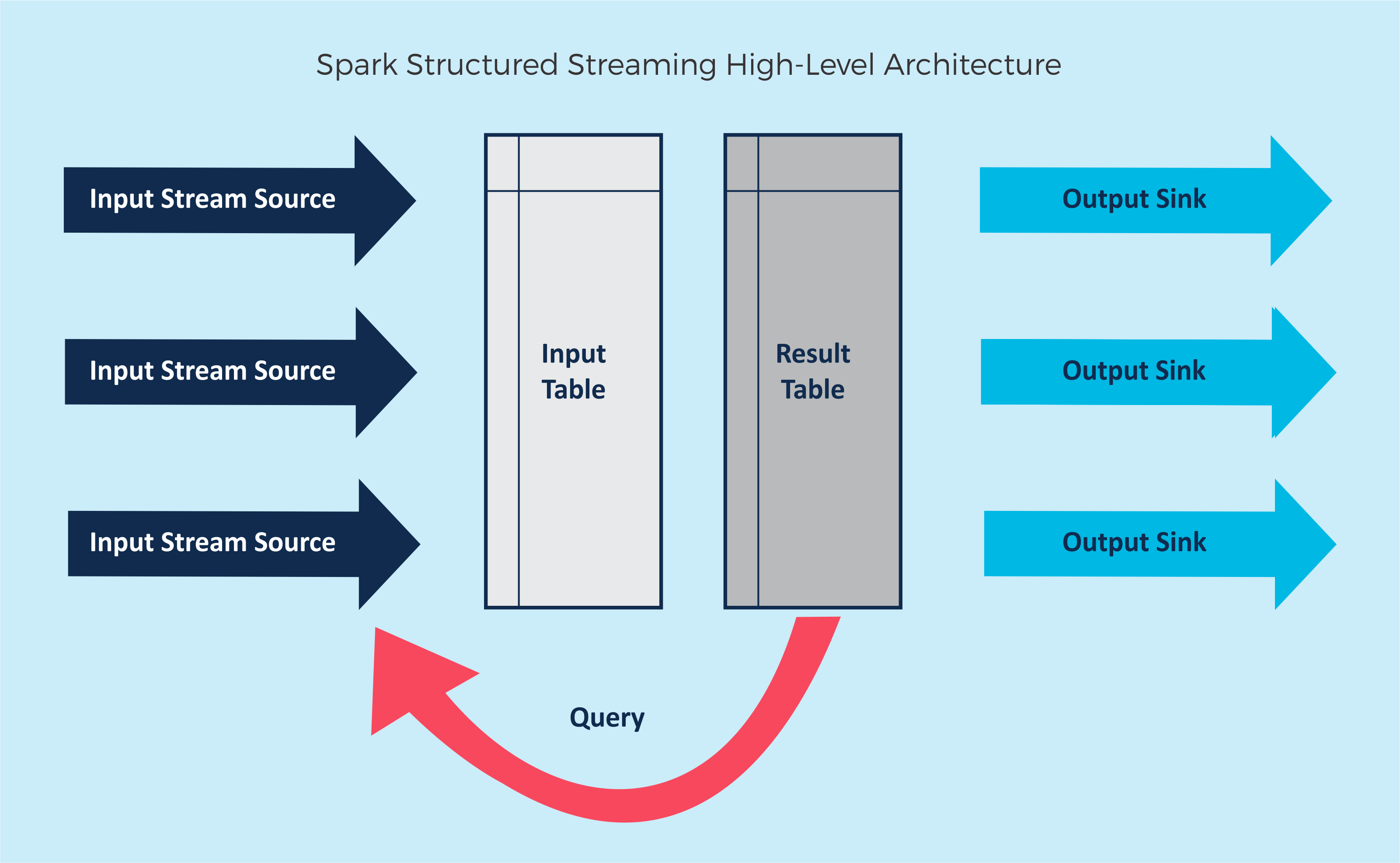
Spark Structured Streaming – Apache Spark Structured Streaming High-Level Architecture
The inbuilt streaming sources are FileStreamSource, Kafka Source, TextSocketSource, and MemoryStream. The last two are only recommended for testing as they are not fault-tolerant, and we’ll use the MemoryStream for our example, which oddly isn’t documented in the main documents here.
Spark structured streaming can provide fault-tolerant end-to-end exactly-once semantics using checkpointing in the engine. However, the streaming sinks must be idempotent for handling reprocessing, and sources must be “replayable” – sockets and memory streams aren’t replayable.
How do we add a streaming data source to a DataFrame? Simply replace inSeq in the above code with an input MemoryStream like this:
val rawIn = MemoryStream[Raw]
val inDF = rawIn.toDF
Note that once a DataFrame has a streaming data source it cannot be treated as a normal DataFrame, and you get an error saying:
org.apache.spark.sql.AnalysisException: Queries with streaming sources must be executed with writeStream.start();
And now put the streaming window function back in:
|
1 2 3 4 5 6 7 8 9 |
val outSLA = inDF .withColumn("time", current_timestamp()) .filter($"service" === "s1" || $"service" === "s2") .withColumn("window", window($"time", windowDuration, slideDuration)) .groupBy("node", "window") .pivot("service") .agg(min("metric"), avg("metric"), max("metric")) .filter($"s1_avg(metric)" > 3 && $"s2_max(metric)" > 1) .select("node", "window") |
The final abstraction we need to add is a “query”, which requires options for output mode, an output sink, query name, trigger interval, checkpoint, etc. The query can then be started as follows:
|
1 |
val querySLA = outSLA.writeStream.outputMode("complete").format("memory").queryName("sla1").start |
Even though Streaming operations can be written as if they are just DataFrames on a static bounded table, Spark actually runs them as an incremental query on an unbounded input table. Every time the query is run (determined by the Trigger interval option), any new rows that have arrived on the input stream will be added to the input table, computations will be updated, and the results will be updated. The changed results can then be written to an external sink.
There are three write modes: Complete, Update and Append (default), but only some are applicable depending on the DataFrame operations used. You can optionally specify a trigger interval. If the trigger interval is not specified the query will be run as fast as possible (new data will be checked as soon as the previous query has been completed). The syntax for providing an optional trigger time is:
.trigger(ProcessingTime(“10 seconds”))
For this example, we used the simple Memory Sink (which is for debugging only). For production, a different sink should be used, for example, a Cassandra sink. For production, a real input stream will be needed. Kafka is a good choice, see the Instaclustr Spark Streaming, Kafka, and Cassandra Tutorial.
Did the streaming code actually work? Not exactly. There is some “fine print” in the documentation about unsupported operators. The list isn’t explicit and sometimes you will have to wait for a run-time error to find out if there’s a problem. For example, the above code didn’t run (and the error message didn’t help), but by a process of trial and error I worked out that pivot isn’t supported. Here’s a workaround, assuming you know in advance which service names need to be aggregated for model prediction input (I used the spark sql when function in the agg to check for each required service name):
|
1 2 3 4 5 6 7 8 9 10 11 |
val outSLA = inDF .withColumn("time", current_timestamp()) .filter($"service" === "s1" || $"service" === "s2") .withColumn("window", window($"time", windowDuration, slideDuration)) .groupBy("node", "window") .agg( avg(when($"service" === "s1", $"metric")).alias("s1_avg"), max(when($"service" === "s2", $"metric")).alias("s2_max") ) .filter($"s1_avg" > 3 && $"s2_max" > 1) .select("node", "window") |
Start Your Streams!
Once a query is started it runs continuously in the background, automatically checking for new input data and updating the input table, computations, and results table. You can have as many queries as you like running at once, and queries can be managed (e.g. find, check and stop queries). Note that stop appears to result in the data in the input sink vanishing (logically I guess as the data has already been read once!)
Is that it? Well not exactly. What’s missing? You will notice that we don’t have any input data yet, and no way of checking the results! The addData() method is used to add input rows to the MemoryStream:
rawIn.addData(Raw(“n1”, “s1”, 3.14))
This is cool for testing. Just add some data, and then look at the result table (see below) to check what’s happened! But It is tedious to create a large data set for testing like this, so here’s the code I used to create more torrential and realistic input data:
|
1 2 3 4 5 6 7 8 9 10 11 12 13 14 15 16 |
import scala.util._ val numNodes = 10 val numServices = 10 val maxValue = 1000000.0 val maxDelay = 100 // add 1000 random events to input stream for (a <- 1 to 1000) { var node:String = "node"+Random.nextInt(numNodes) var service:String = "metric"+Random.nextInt(numServices) var metric:Double = Random.nextDouble*maxValue rawIn.addData(Raw(node, service, metric)) Thread.sleep(Random.nextInt(maxDelay)) } |
(Note that for the final version of the code the names “nodeX” and “serviceX” were used instead of “nX” and “sX”).
Finally, here’s the code to inspect the results. “sla1” is the queryName from the query started above, and processAllAvailable()is only used for testing as it may block with real streaming data, see documentation:
val slaTable = spark.table(“sla1”).as[(String, String)]
querySLA.processAllAvailable()
slaTable.show
One potential issue with streaming data and small sliding window times is data quality and quantity. I.e. there may be insufficient data in a window to compute aggregations to justify an SLA violation prediction. A simple hack is to include a count of the number of measurements in the window as follows:
|
1 2 3 4 5 6 7 8 9 10 11 12 13 14 |
val outSLA = inDF .withColumn("time", current_timestamp()) .filter($"service" === "metric1" || $"service" === "metric2") .withColumn("window", window($"time", windowDuration, slideDuration)) .groupBy("node", "window") .agg( avg(when($"service" === "metric1", $"metric")).alias("metric1_avg"), max(when($"service" === "metric2", $"metric")).alias("metric2_max"), // add count column for data quality check count("*").alias("count") ) // only report SLA prediction is >= 10 measurements .filter($"count" >= 10 && $"metric1_avg" > 6000000 && $"metric2_max" > 9000000) .select("node", "window") |
Here are some results (with avg and max and count cols left in for debugging). Note that because there are 10 windows for each minute of events (as sliding duration was 1 minute) there may be multiple SLA warnings for the same node):
|
1 2 3 4 5 6 7 8 9 10 11 12 13 14 15 16 17 |
slaTable.sort($"window".desc).show +-----+--------------------+------------------+-----------------+-----+ | node| window| metric1_avg| metric2_max|count| +-----+--------------------+------------------+-----------------+-----+ |node8|[2017-10-31 00:41...|6249168.4604176665|9310424.035530351| 20| |node9|[2017-10-31 00:32...|8341091.5492284065| 9047374.18783093| 13| |node8|[2017-10-31 00:33...|6249168.4604176665|9310424.035530351| 20| |node8|[2017-10-31 00:35...|6249168.4604176665|9310424.035530351| 20| |node8|[2017-10-31 00:34...|6249168.4604176665|9310424.035530351| 20| |node8|[2017-10-31 00:39...|6249168.4604176665|9310424.035530351| 20| |node8|[2017-10-31 00:38...|6249168.4604176665|9310424.035530351| 20| |node8|[2017-10-31 00:40...|6249168.4604176665|9310424.035530351| 20| |node6|[2017-10-31 00:41...| 6283795.595735676|9762914.964495799| 16| |node8|[2017-10-31 00:36...|6249168.4604176665|9310424.035530351| 20| |node8|[2017-10-31 00:37...|6249168.4604176665|9310424.035530351| 20| +-----+--------------------+------------------+-----------------+-----+ |
Even after debugging the static pure DataFrame version of the code, there were still a few surprises. One useful trick for debugging is to run multiple streaming queries. One query produces the final results, but other queries can be used to show intermediate steps. For example, use another query to look at the partially processed raw input data (after adding the window):
|
1 2 3 4 5 6 7 8 9 10 11 12 13 |
val debugQuery = inDF .withColumn("time", current_timestamp()) .filter($"service" === "metric1" || $"service" === "metric2") .withColumn("window", window($"time", windowDuration, slideDuration)) .writeStream .outputMode("complete") .format("memory") .queryName("debug1") .start val debugTable = spark.table("debug1").as[(String, String, String, String, Double)] debugQuery.processAllAvailable() debugTable.show |
A cool Zeppelin fact. I discovered a new Zeppelin trick while debugging this code. There’s an implicit Zeppelin context available (called “z”!) which provides a few tricks. For example, a nicer version of the show has options for different types of graphs. Just type “z.show(DataFrameName)”.
3. Triggers, Slides, and Windows
Triggers, Slides, and Windows sound like a risky combination?! I realised I’d glossed over the treatment of time in Spark Streaming, so here’s another attempt at trying to explain how “time works” (at least at a high level).
Trigger time: Rate at which new input data is added to the input table from the input source stream. The default is that after the query is finished it just looks again.
Sliding duration: How often the window slides (possibly resulting in some events being added or removed from the window if they no longer fall within the window interval).
Window duration: The duration of the window, determines the start and end time (end-start = window).
The following 3 diagrams illustrate three cases. Example 1 has a trigger time of 1 (unit of time), a slide of 1, and a window of 10. The timeline is at the top (from 1 to 17), and one event arrives during each period of time (a, b, c, etc). Events are added to the input table once per trigger duration, resulting in one event being added each unit time in this example. Multiple sliding windows are created, each is 10 time units long, and 1 unit apart. After 10 time units, the 1st window has 10 events (a-j) and then doesn’t grow any further. The 2nd window (which started 1 time unit later than the 1st) contains events b-k, etc.
Example 2 shows what happens if the trigger time (2 time units) is longer than the sliding time (1 time unit). This results in a potential backlog of events, with all the events that have arrived on the input stream since the last trigger being added to the window at the next trigger time (in this case we get both events a and b added during the time 2 period, c and d during period 4, etc.).
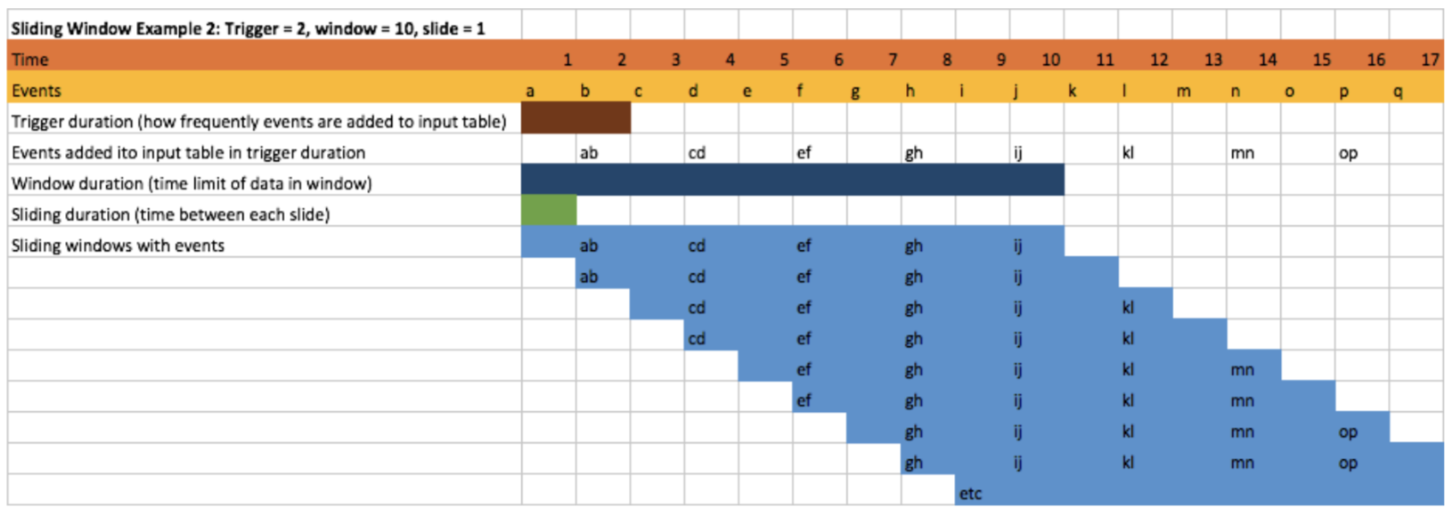
Triggers, Slides and Windows Apache Spark Example 2
Example 3 shows a Tumbling window when the sliding and window times are equal (5 units):
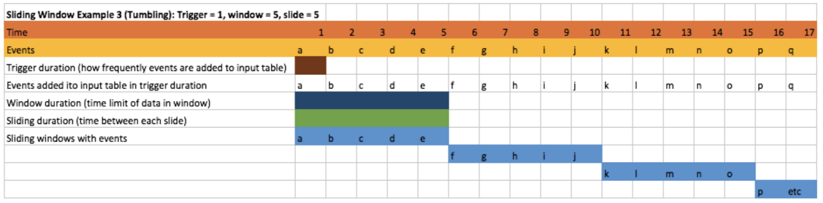
Triggers, Slides, and Windows Apache Spark Example 3
What are sensible defaults for these times? Trigger time <= Slide time <= Window duration.
Is there anything wrong with having a very short trigger or sliding times? Short trigger times may increase resource usage (as the query must be re-run over each new input event), and short sliding times will increase the number of concurrent windows that need to be managed. Long window times may increase the amount of data and processing required for each window. I.e. more frequent and larger computations will consume memory and CPU.
However, the actual times will need to be determined based on your use case, taking into account the data velocity and volumes and the time-scales of the “physical” system being monitored and managed.
Also (as we noticed from the example output), sliding windows will overlap each other, and each event can be in more than one window. “Tumbling” windows don’t overlap (i.e. duration and sliding intervals are the same). If no sliding duration is provided in the window() function you get a tumbling window by default (slide time equal to duration time). Which sort of window do you need? For the same use cases, the data must not (or just don’t need to be overlapping), so a tumbling window must be used is applicable (e.g. periodic report generation such as a daily summary) For other applications it’s important to have more frequent updates but still a longer period (the window time) for computing over, so sliding windows are the answer.
The location of the window() function documentation isn’t obvious. It’s in the org.apache.spark.sql.functions package, spark sql streaming window() function documentation. The parameters windowDuration and slideDuration are strings, with valid durations defined in org.apache.spark.unsafe.types.CalendarInterval. In theory, durations can range from microseconds to years, although using units greater than weeks produces an exception, probably so that you don’t accidentally have a window with too much data in it. Durations greater than months can be specified using units less than months (e.g. “52 weeks”). Long windows can make sense when the timespan of the data is long but the quantity of data is manageable, otherwise, batch processing may be preferable. Also, note that slideDuration must be <= windowDuration.
|
1 2 3 4 5 6 7 8 9 10 11 12 13 14 15 16 17 18 19 20 21 22 23 24 25 26 27 28 29 30 31 32 33 34 35 36 37 38 39 40 41 42 43 44 45 46 47 48 49 50 51 52 53 54 55 56 57 58 59 60 61 62 63 64 65 66 67 68 69 70 71 72 73 74 75 76 77 78 79 80 81 82 83 84 85 86 87 88 89 90 91 |
// complete commented code including imports import spark.implicits._ import org.apache.spark.sql.functions._ import org.apache.spark.sql.execution.streaming.MemoryStream import org.apache.spark.sql.streaming.{OutputMode, Trigger} import org.apache.spark.sql.functions.{sum, when} import scala.util._ import scala.concurrent.duration._ import org.apache.spark.sql.SparkSession val spark: SparkSession = SparkSession.builder.getOrCreate() implicit val ctx = spark.sqlContext // how much data to retain in window // note that the time is a String! What units are allowed? val windowDuration = "10 minutes” // how often to update the data // defaults to windowDuration if not supplied val slideDuration = "1 minutes" // class for raw data: (node, service, metric) // what’s the case for? Look at the docs: // https://docs.scala-lang.org/tour/case-classes.html case class Raw(node: String, service: String, metric: Double) // Seq of sample input data for testing val inSeq = Seq( Raw("n1", "s1", 1.0), Raw("n1", "s1", 10.0), Raw("n1", "s2", 2.0), Raw("n2", "s1", 33.0) ) // turn into DataFrame val inDF = inSeq.toDF() // DataFrame transformations to turn raw input data into: // prediction of SLA violation for (node, window) val outSLA = inDF // raw data didn’t have a timestamp (event-time), // so add processing-time timestamp as new “time” column .withColumn("time", current_timestamp()) // assume that our model only uses a subset of a potentially // large number of metrics, and we know what they are. // filter on them early so we can throw away lots of data // retain only rows with metric names equal to s1 or s2. .filter($"service" === "s1" || $"service" === "s2") // add a new column called “window” which is a window // i.e. a start and end timestamp, using the window function // applied to the time column, with specified window and slide // times .withColumn("window", window($"time", windowDuration, slideDuration)) // Whoops, doesn’t work for DataFrame code, replace test hack: // .withColumn("window", $"time") // next 3 operations need to be used together and will // produce a wide-table: // groupBy: with a single row for each unique window+node permutation, // pivot and agg: for each unique service name 3 new columns will be created for min, avg, and max of the value of the service (metric) computed over the window+node+service values .groupBy("node", "window") .pivot("service") .agg(min("metric"), avg("metric"), max("metric")) // stand-in code for MLLib model prediction function. // Assuming we previously produced a decision tree model // it’s easy to extract the logic for the positive label // prediction and turn it into a filter for a demo. // Returns rows which are predicted to have a SLA violation // next time period .filter($"s1_avg(metric)" > 3 && $"s2_max(metric)" > 1) // select node and window columns (for debugging better to // return all columns .select("node", "window") // start a query to write to a memory sink with queryName “sla1” // use outputMode “complete” and default trigger interval // the syntax for proving a trigger time as follows: // .trigger(ProcessingTime("10 seconds")) val querySLA = outSLA.writeStream.outputMode("complete").format("memory").queryName("sla1").start |