A Kafka performance model for SSDs/EBS, network, I/O, and brokers
In Part 1 of this new series, we explored the question: how do you resize a Kafka cluster (using Solid State Drives [SSDs] for local storage) for producer and consumer workloads on topics with remote Tiered Storage enabled?
Now in Part 2, we’re going to explore a Kafka performance model for SSDs/EBS, network, I/O and brokers!
Not all Apache Kafka® clusters use SSDs (Solid State Drives) for local storage. In fact, some of our biggest Kafka clusters opt for AWS Elastic Block Store (EBS) for local storage instead (they can be SSDs or HDDs [hard disk drives] but connected to Kafka brokers via a network).
The “Elastic” in EBS also gives our customers the ability to resize their NetApp Instaclustr Kafka clusters. I’ve also previously used an EBS-backed Kafka cluster to achieve 19 Billion anomaly checks per day for a massively scalable demonstration application (Anomalia Machina), scaling the “Kongo” (IoT) application on a production cluster, and benchmarking for The Power of Apache Kafka Partitions.
The main difference we now need to include in our Kafka Tiered Storage performance model is that writes to and reads from EBS storage all occur over a network rather than local I/O (so they are similar to remote storage workloads in our Tiered Storage model in that respect).

Continuing the “cheese” theme from the previous blog, let’s try some stretchy “elastic” cheese (fondue)!
(Source: Adobe Stock)
1. EBS and Tiered Storage enabled
Here’s the amended complete Kafka Tiered Storage model for EBS local storage. I’ve added a new internal component for the total EBS network bandwidth (to and from EBS storage from the Kafka cluster, EBSNet).
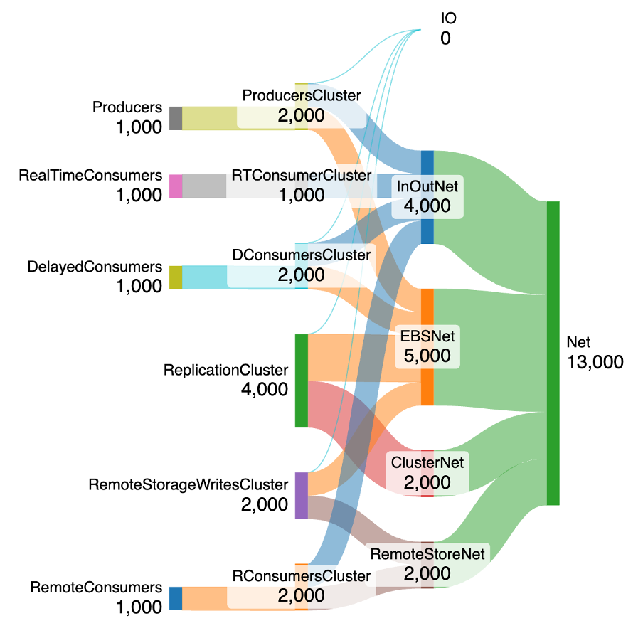
The main obvious difference to the previous SSD model is that there’s no load on the cluster I/O anymore (there is no “local” storage attached directly to the Kafka brokers), the new EBS Network load is 5,000 MB/s, and the total Network load has increased to 13,000 MB/s. This is the “default” scenario with a 1,000 MB/s producer workload, fan-out of 3, and an equal split for each type of consumer workload (real-time, delayed, and remote).
2. EBS and Tiered Storage disabled
Now let’s keep the EBS local storage but disable the Tiered Storage for comparison (representing the initial cluster before resizing for tiered remote storage). The producer workload is still 1,000 MB/s, but real-time and delayed consumer workloads have a 50:50 split still resulting in a fan-out of 3.

The EBS Network load has reduced to 4,500 MB/s and the total Network load is 10,500 MB/s.

Comparing cheeses! (Source: Adobe Stock)
3. Comparing SSDs vs. EBS and remote Tiered Storage enabled vs. disabled
Let’s now summarize our findings so far with the following graphs comparing SSD/EBS and remote Tiered Storage enabled and disabled for the default workloads and the x10 remote consumer workloads (see previous blog):
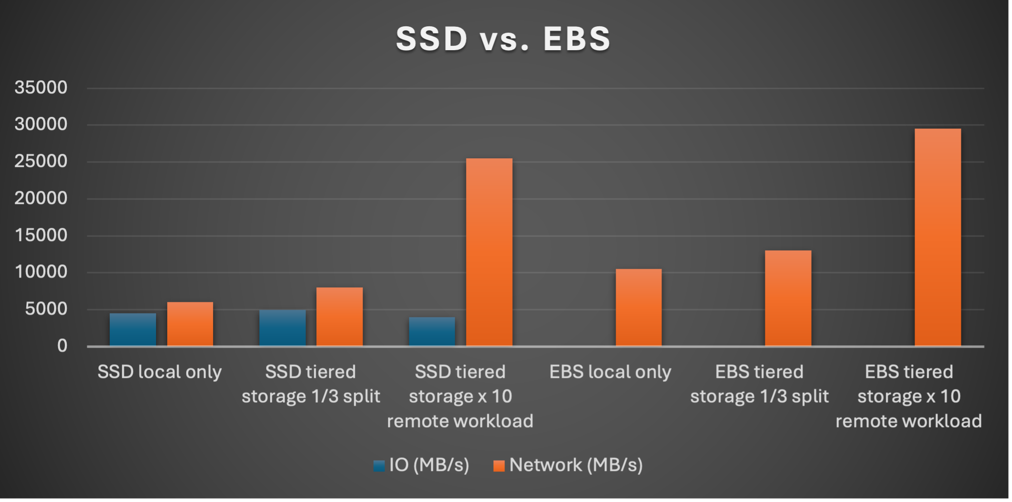
What do we notice?
Naturally, there’s no I/O demand for the EBS scenarios (as local storage is networked). As we noted in the last blog, enabling Tiered Storage for SSDs increases the network bandwidth (+33%), and the absolute network load is higher for the EBS scenarios as everything happens over the network. However, the percentage increase is smaller (+23% for EBS tiered c.f. local).
4. How many brokers does the cluster need?

Which type and how much cheese do you need? (Source: Adobe Stock)
The NetApp Instaclustr Kafka team regularly runs Kafka benchmarks on Kafka clusters composed of different AWS instance types and sizes, so I had a look at the most recent results and discovered a few things that may be relevant for Kafka Tiered Storage modelling and prediction including:
- A subset of the instance types and sizes that we benchmark are:
- AWS R6g, large to 2xlarge (2 to 8 vCPUs)
- These support EBS for the local storage
- AWS i3 and i3en (xlarge to 2xlarge, 4 to 8 vCPUs)
- These include NVMe SSDs for the local storage
- AWS R6g, large to 2xlarge (2 to 8 vCPUs)
- Test results include the “baseline” network bandwidth, and actual network bandwidth, throughput achieved, I/O wait (< 5% for a successful run) and CPU utilisation (< 50% for a successful run).
- The maximum measured network bandwidth achieved is typically around 70-80% of the “baseline” bandwidth.
- Larger instances consistently provide more CPU and network, but not necessarily more I/O.
So, with this information as a starting point, I asked our team a few more questions and they pointed me to the AWS EC2 specifications. This page (and sub-pages for the different EC2 Categories) provides more complete information on the capacity of each instance type and size. I looked up the instances above and found that R6g instances are:
- memory optimized
- use AWS Graviton2 Processors
- have only 1 thread per core
- have a baseline network bandwidth (minimum)
- and a burst bandwidth (maximum)
- and include dedicated baseline and burst network and I/O for the EBS storage.
Given that the burst capacity is only available for relatively short periods of time, we will rely on the baseline values for modelling and prediction.
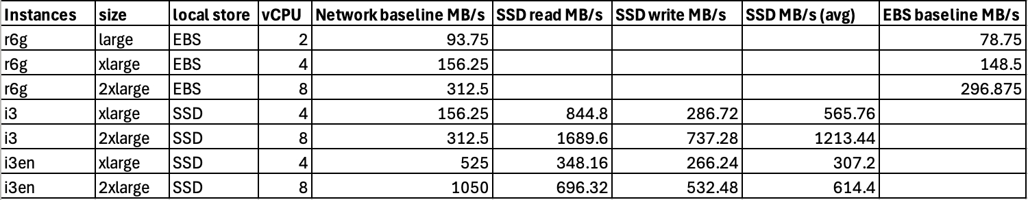
AWS i3 (Xen hypervisor) and i3en (Nitro v3 hypervisor) are storage optimised instance types. I3 instances are Intel Broadwell E5-2686v4 processors (2 threads per core) and i3en are Intel Xeon Platinum 8175 processors (also 2 threads per core). They also have baseline/burst network bandwidths but are designed for SSDs and include specifications for SSD sizes and read/write IOPs (from which throughput for 4k byte block sizes can be estimated)—reads are faster than writes.
A summary of this information is in the following table:
By adding this information to the Kafka performance model (for the default scenario), we can now compute the minimum number of brokers required to satisfy the total I/O and Network demands on the Kafka cluster, taking into account which resource is the first bottleneck encountered. Here are the results comparing local-only storage vs. remote Tiered Storage enabled:
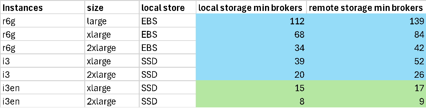
The bottleneck for the blue highlighted results is the network, but for the green results (i3en) the bottleneck is SSD I/O (the prediction is the minimum number of brokers of each type/size for the I/O, so there’s more Network capacity spare). The potential increase in brokers is from 24% to 33 % more for networked limited clusters (blue), and 13% more for I/O limited clusters (green).
Also please note that:
- Because the current model doesn’t compute separate write and read SSD loads, and I averaged the SSD write/read IOPs capacity, these results are only approximate.
- You will also need to increase these estimates by 20 to 30% to allow for the 70-80% maximum network bandwidth utilisation we obtained with our internal benchmarks.
- You can choose to use average or peak workload rates, but the resource estimates will naturally increase substantially for peak workloads (and depending on how long the peaks last, you may have sufficient burst credits to cover the increased resource demand, or not).
- The model doesn’t take into account CPU utilization, yet which is likely to be more with Tiered Storage enabled.
- These are purely predictions of the absolute minimum cluster wide I/O and Network demands – your existing cluster may already have these to spare, and therefore be “bigger” (more/bigger brokers) than this, due to disk storage and/or CPU requirements etc.
- Finally, these results are just general guidelines. For more specific and customised predictions, the model needs to be parameterized with actual workloads, fan-out ratio, and percentage of topics that have Tiered Storage enabled, etc.
The potential savings for Tiered Storage vs local storage are also likely to be substantial, but that will depend on the retention settings, throughputs, and local storage type (SSD vs. EBS) etc–we will explore the storage trade-offs and costs in the next blog.
Update! I’ve put some of the functionality from the Excel/Sankey Diagram model (not including broker types/sizes) into a prototype JavaScript/HTML Kafka sizing model available on GitHub. This includes producer and consumer workloads, SSD or EBS, RF, and Tiered Storage enabled/disabled, and predicts and graphs total Kafka cluster I/O and Network bandwidth loads, and fan-out ratio – enjoy!
======
And now for a final historical “cheese” related capacity/sizing fact! How much cheese (or rabbits or eggs) could you fit in a South Australian Railways refrigerator (‘R’) car?
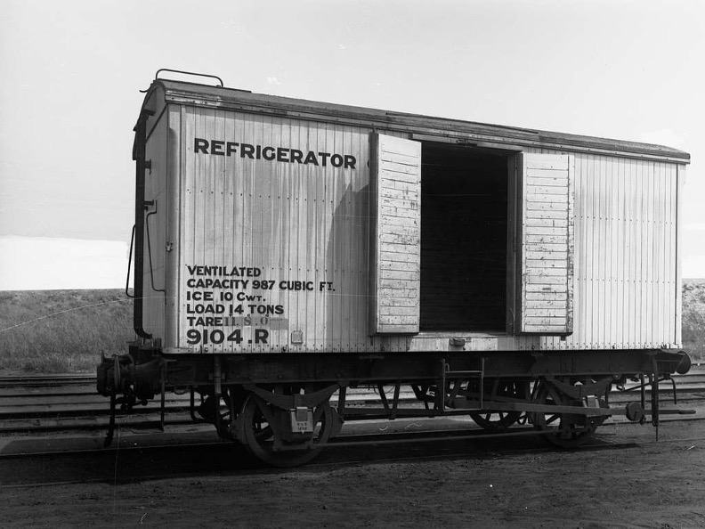
(Source: The History Trust of South Australia, South Australian Government Photo, CC0)
Well, back in the day, you could load 261 boxes of cheese in an ‘R’ car, or 420 boxes of rabbits, or 336 boxes of eggs! Or even overload them by 10% (but only in South Australia!)
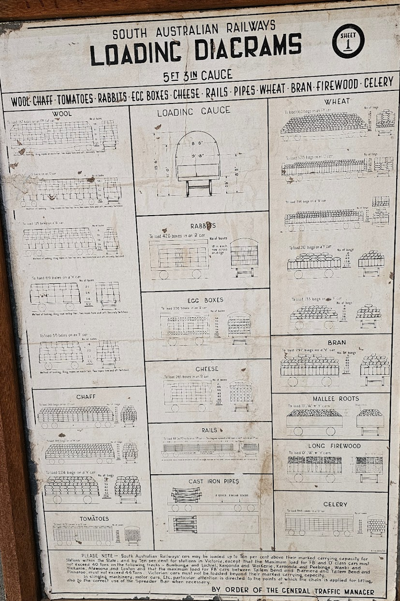
Peterborough Railway Museum, SA Railways car loading regulation (Source: Paul Brebner)
Follow along in the How to size Apache Kafka clusters for Tiered Storage series…
And check out my companion series, Why is Apache Kafka Tiered Storage more like a dam than a fountain?