What

Bloom filters are space-efficient probabilistic data structures that can yield false positives but not false negatives. They were initially described by Burton Bloom in his 1970 paper  “Space/Time Trade-offs in Hash Coding with Allowable Errors“. They are used in many modern systems including the internals of the Apache® projects Cassandra®, Spark™, Hadoop®, Accumulo®, ORC™, and  Kudu™.

Multidimensional Bloom filters are data structures to search collections of Bloom filters for matches. The simplest implementation of a Multidimensional Bloom filter is a simple list that is iterated over when searching for matches. For small collections (n < 1000) this is the most efficient solution. However, when working with collections at scale other solutions can be more efficient. 

We implemented a multidimensional Bloom filter as a Cassandra secondary index in a project called Blooming Cassandra. The code is released under the Apache License 2.0.  The basic assumption is that the client will construct the Bloom filters and write them to a table. The table will have a BloomingIndex associated with it so that when the Bloom filter column is written or updated the Index will be updated. To search the client constructs a Bloom filter and executes a query with a WHERE clause like WHERE column = bloomFilter.  All potential matches are returned. The client is responsible for filtering out the false positives.

The CQL code would look something like this:

Why

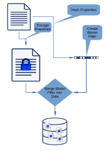
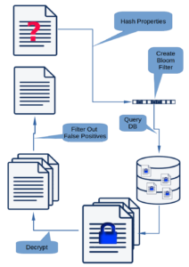
Our initial use case was that we wanted to be able to encrypt data on the client, write the data to Cassandra, and be able to search for the data without decrypting it. Our solution is to create a Bloom filter comprising the original plain text for each searchable column, encrypt the columns, add a column for the unencrypted Bloom filter, and write the resulting row to Cassandra. To retrieve the data, the desired unencrypted column values are used to create a Bloom filter. The database is then searched for matching filters and the encrypted data returned. The encrypted data are decrypted and false positives removed from the solution. This strategy was presented in my 2020 FOSDEM talk “Indexing Encrypted Data Using Bloom Filters”.

The Bloom filter could also be used to produce a weak reference to another Cassandra table to simplify joins. If we assume two tables: A and B where there is a one-to-many correspondence between them such that a row in A is associated with multiple rows in B. A Bloom filter can be created from the key value from A and inserted into B. Now we can query B for all rows that match A. We will have to filter out false positives, but the search will be reasonably fast.

With the multidimensional Bloom filter index, it becomes feasible to query multiple columns in large scale data sets. If we have a table with a large number of columns, for example, DrugBank; a dataset that contains 107 data fields, a column could be added to each row comprising the values for each data field. Then queries could be constructed that looked for specific value combinations across those columns.

How

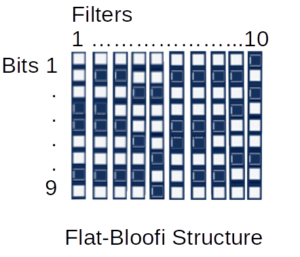
Several multidimensional Bloom filter strategies were tried before the Flat-Bloofi solution was selected.  Flat-Bloofi as described by Adina Crainiceanu and Daniel Lemire in their 2015 paper “Bloofi: Multidimensional Bloom filters“, uses a matrix approach where each bit position in the Bloom filter is a column and each Bloom filter is a row in a matrix. To find matching bloom filters for a target filter, each column of the matrix that corresponds to an enabled bit in the target is scanned and the row indexes of all the rows that have that bit enabled are collected into a set. The intersection of the sets is the set of Bloom filters that match.

We also tested a “Chunked Flat-Bloofi” which breaks the filter down by bytes rather than bits.  This solution worked well for small data sets (n<2 million rows), however, the query process suffers from a query expansion during the search as described below. On storage, the Bloom filter is decomposed to a byte array and each non-zero byte, its array position and the identifier for the Bloom filter is then written to an index table. When searching for the target, the target Bloom filter is decomposed to a byte array and each non-zero byte is expanded to the set of all “matching” bytes, where “matching” is defined as the Bloom filter matching algorithm. The index table is then queried for all identifiers associated with the matching bytes at the index position. The result of this query is the set of all Bloom filters that have the bits enabled in the target byte and position. Each set represents a partial solution, the complete solution is the intersection of the sets. The solution is the complete set of matching identifiers.

The query expansion problem occurs whenever a Multidimensional Bloom filter strategy uses chunks rather than bits as the fundamental query block. Each target byte, with the exception of 0xFF, has more than one matching solution. For example the byte 0xF1  will match 0xF1 , 0xF3 , 0xF5 , 0xF7 , 0xF9 , 0xFB , 0xFD  and 0xFF . This has to be accounted for in the query processing or the original indexing.

The Flat-Bloofi implementation was built using memory mapped files to allow for fast access to the data. The implementation comprises 4 files, the Flat-Bloofi data structure, a list of active/inactive elements in the Flat-Bloofi structure, a mapping of the Flat-Bloofi numerical ID to the data table key, and a list of active/inactive mapping entries. The standard SSTable index was used to map the data table key to the Flat-Bloofi id.  All code is available in the Blooming Cassandra code base.