Fantasy Basketball.
Part statistics, part unpredictable human behaviour.
It works like this: All the players in the NBA are put into a pool. Then, all the fantasy team owners take turns drafting the NBA players onto their fantasy team, building up the team. Then, each week, two teams go head to head, competing to see who can win more categories.
For the last two seasons, I have watched another player lift the trophy in my Fantasy Basketball league. I have watched as my team sat on the sideline in the final week, jealous that I hadn’t picked the right players in the draft, or that I had made bad trades. I recently found out that I placed 11th out of the 12 teams in the draft order, and I was sick of losing.
So taking after the latest trend in sports, I decided I would need to explore the statistics.
This presented a huge hurdle for me. I am horrible at the statistics. I find it hard to visualise the data, and easily get overwhelmed by the calculations. The closest I ever came to failing a course was first year statistics. So I knew that I needed help. Lucky for me, I had recently been playing around with Elassandra, and Kibana, which would (hopefully) make it easier for me to get the data I needed.
Fantasy Basketball 101:
To follow this blog, you might need to understand a little more about fantasy basketball (and maybe basketball to begin with).
The Scoring System
The scoring system is based on the real-life statistics NBA players score. Each week the statistics of each player go to the fantasy team which “owns” them. Say you draft James Harden, and he scores 31 points, 11 assists, and 8 rebounds. This means your fantasy team gets 31 points, 11 assists, and 8 rebounds. This happens for each game each player on your team participates in, for the whole week. You own a player either by drafting or trading them.
In the league I play in, there are 11 categories:
- PTS (Points which the player scores)
- REB (Rebounds the player collects)
- AST (Assists the player makes)
- STL (Steals the player makes)
- BLK (Blocks the player makes)
- TO (Turnovers – the only statistic where the goal is to have less)
- FG% (Field Goal percentage – Total shots made / total shots attempted (free throws not included))
- FT% (Free throw percentage – Total free throws made / total free throws attempted)
- 3P% (Three point percentage – Total 3 point shots made / total 3 point shots attempted
- 3PM (Three point shots made)
- DD (Double doubles – scoring double digits in two of the first 5 categories)
GOAL: Win 6 (or more) categories against your opponent each week. If you can achieve that, you “win the week”.
The Draft Process
Each year, we randomly generate the draft order for the 12 teams. This dictates which order you will be drafting. Teams draft 13 players for their team. Obviously this would be unfair if the Team which got the #1 pick, also picked 13th, so we do what’s called a “snake draft”. That means that the player that gets the 12th pick, also gets the 13th pick, the player who gets the 11th pick also gets the 14th pick (and we count backwards from there back to 1, then back to 12, then backwards down to 1).
Punting Categories
This is a strategy by where you intentionally ignore certain categories. You get the same number of points if you win 11 categories each week as if you win 6, so why try and win as many as possible? Maybe you should just focus on winning 6 specific categories. This means that players which have “warts” – categories in which they are significantly worse than average – are undervalued when compared to your punting strategy. If you are punting Free Throw % and 3P%, then your strategy will value players with these particular deficiencies higher than normal. Given that I was picking later in the draft, I thought that punting categories may give me the advantage I needed.
The Technical Fun
Technology Choice
Given that I didn’t know what I was looking for, I wanted to use something that I could use to perform some data exploration, and hopefully get more information. Kibana and the Elasticsearch API fit this perfectly. It would allow me to load in last seasons statistics, the predicted statistics for next season, and perform all kinds of queries and graphing on it.
Creating the Cluster
First thing I did, was starting up an Elassandra cluster with Instaclustr. Given that we would only have a small dataset, and I wasn’t too phased about performance, I selected the t2.micro node size. Also, to make things easier, let’s create it in the US East 1 region of AWS, turn off Password Authorization, and make sure to add your ip to the allowed Elasticsearch, Kibana, and Cassandra ip’s. Making a note of my cluster ips, usernames, and passwords (located on the connection info page), I started the data exploration adventure.
Player Data
So first step – we need to import the data into the Elassandra cluster, but what data do we want to analyse.
Given that we had 12 teams, and 13 players per team, I decided to use the top 150 players in the ESPN orderings. It’s a little less than the 156 players who will be drafted, but it’s really your top 12 players that count.
I got all the player stats for the last year, and the ESPN predictions for next year, and put it into the cluster. For Rookies (players who didn’t play last year) I used their ESPN predictions, and their college statistics for categories I needed. Obviously, this isn’t perfect, but with less than 10 rookies in the top 150, I decided it wasn’t worth worrying about too much.
For most categories, we simply input the category value, but for the percentage based categories (FT%, FG%, and 3P%) we need to weight the percentages, based on how much someone shoots. The idea being that someone who as shoots a lot badly, is worse than someone who shoots very bad, but only takes 1 shot a game. To do this we multiply attempts per game by percentage.
Getting it Into Elassandra
To start with, grab a copy of the example code from the repository here. All code in the repository is heavily commented, to help you understand what is happening. To install the required dependencies, use ‘pip install -r requirements.txt’. I would recommend doing this inside a python virtual environment.
Now we will start to input the data. All steps here are sequential, you must wait for one to complete before attempting the next one. Inputting the base data into the Elassandra has two main files:
The playerData.csv file stores all the raw player data that we will need for our analysis. This dataset is a mixture of predictions for the 2018 season, and data from last season.
The ImportPlayerData.py file is the one which does all the work here. At a high level, it first creates the elasticsearch index ‘fantasy’. This also creates a corresponding cassandra keyspace ‘fantasy’. It reads in the data from the csv, and writes this data into a new cassandra table ‘player’.
In order to run the import code, let’s run it with
python3 importPlayerData.py -ip “<comma separated list of cluster IPs>” -url “<Elasticsearch URL of your cluster>” -u “elasticsearch password” -p “elasticsearch password” -f “the location of the player data csv”
Data Analytics
First Visualisation – Category Spread
Once this data was imported into Elassandra, I wanted to do my first analysis. I wanted to find out what categories are “top heavy”. That is, are there some categories which are so hard to win, because they are influenced by a small majority of players. These would be the categories I either have to punt, or pick players to ensure I won them. To do this I wanted to do a box plot of each of the 11 statistical categories.
In order to do this, what we are going to do is create a separate mapping, based off the data in the player category. We create a new mapping, categories, and write in all the data in the format we need, for easy searching. This is done in the Categories.py file.
The fantastic thing about Elassandra is, straight away, we can start doing Elasticsearch queries on data we wrote to cassandra, and write straight back to Elasticsearch, which will in turn be readable through Cassandra. So, at a high level, the categories file is going to search for every player, then for each category, write that value back to a new Elasticsearch index ‘category’.
We can run the Categories file using the command:
python3 Categories.py -url “<Elasticsearch URL of your cluster>” -u “elasticsearch password” -p “elasticsearch password”
Then, using Kibana, we can graph the percentiles of each of the categories. So click on the Kibana tab on your cluster, and login using the details on the connection info tab.
Once here:
- Define the default index as ‘fantasy’, untick “Index contains time-based events” and hit create.
- Then head to the ‘visualise’ tab. Then a ‘vertical bar chart’ and ‘from a new search’.
- Click on the drop down arrow next to y axis, and we are going to do a Percentiles search over the values. I’m going to plot the 25, 50, 75, 95 and 100th percentiles.
- Then, under the buckets tab, lets do X-Axis.
- The Aggregation will be by Terms, and then select ‘Category’. Make sure to set the size to 11.
- Also, under options at the top, I’m going to select that the bar mode be percentage.
That should give you the graph below:
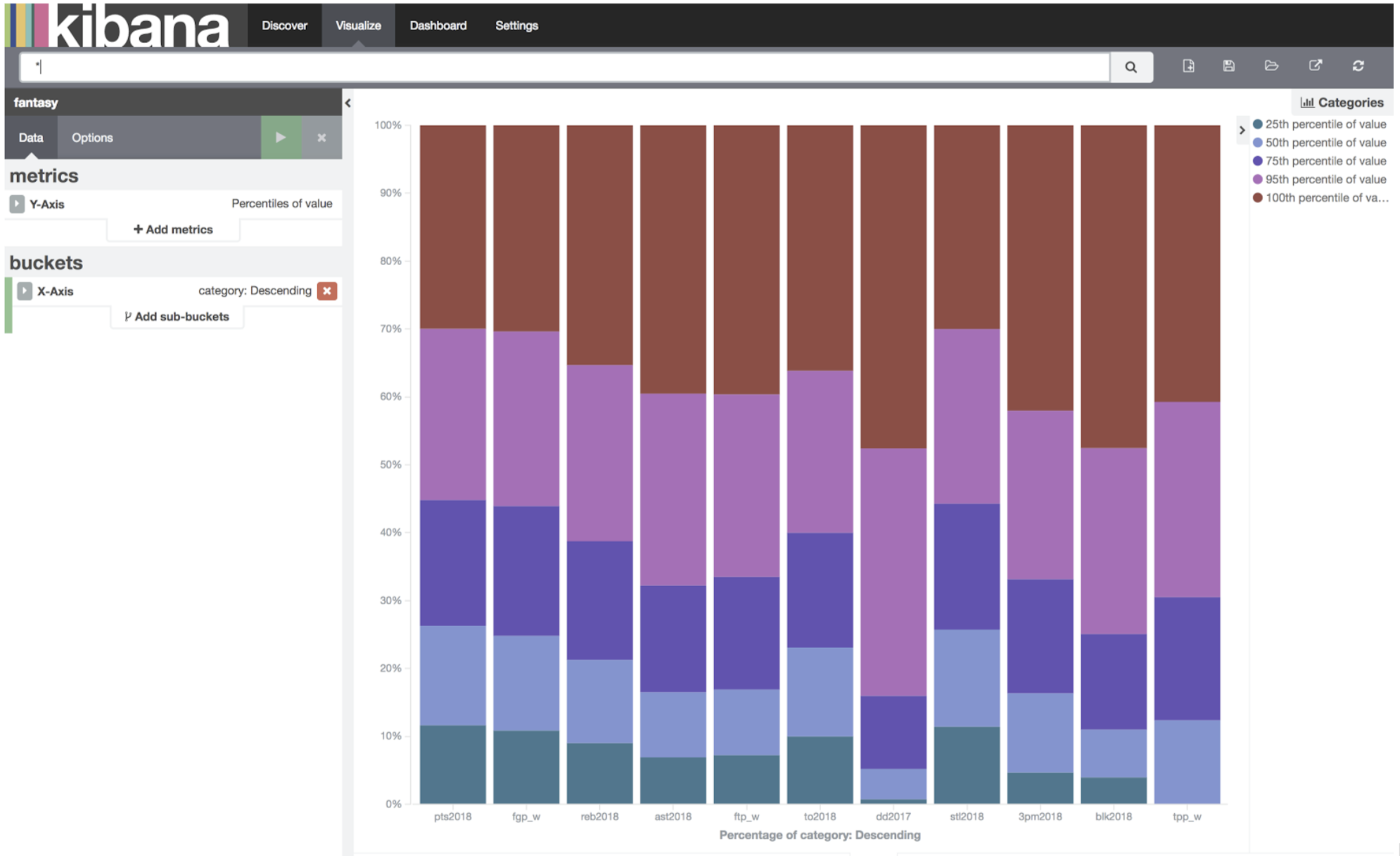
Categories
What we are looking for is categories where the 95th and 100th percentile is the largest size. This means the percentage of the category which is scored by the top 5% (and top 0 players%).
Straight away we can see that DD’s, BLK, TPP, TPM, AST and FGP are probably the categories most likely to be won by a few players. Either we need to win them, or punt them. The other categories, TO, STL, REB, PTS, FTP are categories we will not put heaps of effort towards winning, but hope to get value in the later rounds from them.
Getting averages for each category
This is where we use Elassandra to calculate the averages for each category. Using a quick query, we can get the average of each of the categories we have. Then we write this back into the Elassandra Cluster.
This is done in the averages.py file, where are querying elasticsearch for the average value of specific metrics. Even though we wrote the data into Elassandra through the Cassandra pathway, we still have access to aggregate searches through Elasticsearch. This means that we don’t have to calculate the averages ourselves, but can get Elasticsearch to give it to us through a query.
In order to calculate the averages we can run it with ‘python3 Averages.py -url “<Elasticsearch URL of your cluster>” -u “elasticsearch password” -p “elasticsearch password”’
We then write the averages back into the cluster, it is going to be useful in the next step: my attempt at data analysis.
Player’s Worth
Calculating a player’s worth can be very tricky. One method for calculating a player’s value in real NBA analysis is the WARP statistic. The idea is a player is worth as much as he helps his team, above the average replacement player. This idea intrigued me for Fantasy. By calculating the “average player” on the top 150 players, we can get our own fantasy version of WARP.
So, the basic idea behind my analytics is that the players value, for any given category is (player stat – average stat). This is a good first step. But if we leave it as is, categories like points, where the average is in the mid 30’s, would be weighted significantly more than categories like blocks, which are in the low single digits.
So we will first normalise the values. This would be:
normalised value = (player value – minimum player value) / (maximum player value – minimum player value).
If NBA players were superhumans, sorry – more superhuman then they already are, they would play the full 82 games per year. But the truth is, that players get injured, and miss games. Some players have a history of injuries and are more likely to miss more games. So, we need to weight each category with expected number of games.
Weight = (player expected games /82) – There are 82 games in an NBA season
So putting it all together, each category will be:
player value = Normalised(player statistic) – normalised(average statistic) * (player expected games / 82)
And that’s it – that’s all the statistical talent I have. There is almost certainly a better and more accurate statistical formula for evaluating the player value – but I don’t need 100% accuracy. I need help finding large outliers, and deciding if one player or another is of more value to me with my specific punting categories.
This is all done in the ‘getValues.py’ file, which does all the above, for each category. We can run this with ‘python3 GetValues.py -url “<Elasticsearch URL of your cluster>” -u “elasticsearch password” -p “elasticsearch password”’
Player Value:
To calculate the overall player value, I simply summed all the weighted normalised category values, and wrote this back into Elassandra corresponding with the players name.
To start with, let’s calculate the player’s value by running ‘python3 CalculateValue.py -url “<Elasticsearch URL of your cluster>” -u “elasticsearch password” -p “elasticsearch password”’
Now, because we have added new fields to Elasticsearch, we need to get Kibana to find them. So head back to Kibana and :
- Press the ‘settings’ tab.
- Click on the fantasy index on the left,
- then the yellow ‘refresh fields’ button.
This will scan Elasticsearch for any new fields, like the ones we have just created. We will need to do this step again later, so remember it for when I mention “Refreshing Elasticsearch Fields”.
Now – let’s graph some player value (top 25 players only to start with). This is where I started to see some VERY interesting data.
Now go to ‘visualise’ and:
- Create another vertical bar chart, from a new search.
- We will plot the average ‘player_value’,
- The bucket will be an X-Axis again, aggregate it against the term ‘player name’
- Show the top 25 descending.
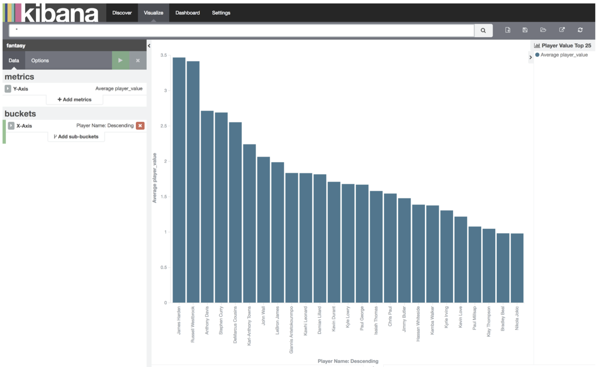
Player Value Top 25
Now you understand why I am so unhappy with the #11 pick. At #11 Damien Lillard is “worth” nearly half of the presumptive #1 pick – James Harden. Great. I’m going to have to go through the bargain basement to win this comp.
Categories with Value
What I’m going to do now is plot the normalised statistical value, against the players, sorted by the ranking by player value. The idea behind this is to try and find which categories I should be punting, and which categories I should be trying to win.
Then, let’s visualise a new line chart, from a new search. We are going to plot the average dif_3pm against the player name, top 25 descending, but sorted by the custom metric, the average ESPN rank, top 25. Then we are going to add all of the remaining 10 categories by pressing “Add Metrics” in the top row and working through them.
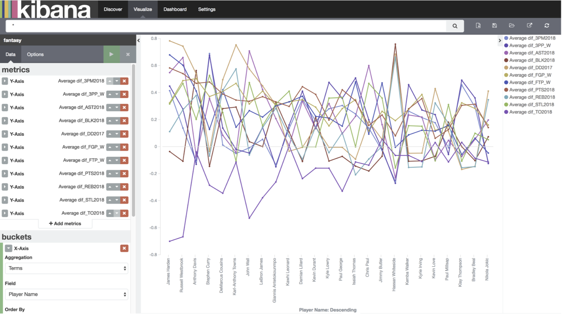
All Categories Top 25
The first thing I notice: How tightly coupled 3PP and 3PM are. This makes sense – good shooters generally shoot more than bad shooters. This means – realistically I either need to punt both categories or go after both categories. Punting one of the two is a bad idea. At this stage, I’m going to punt them.
If we remove all the other categories apart from dif_3PM2018 and dif_3PP_W from the graph, we should get the following graph:
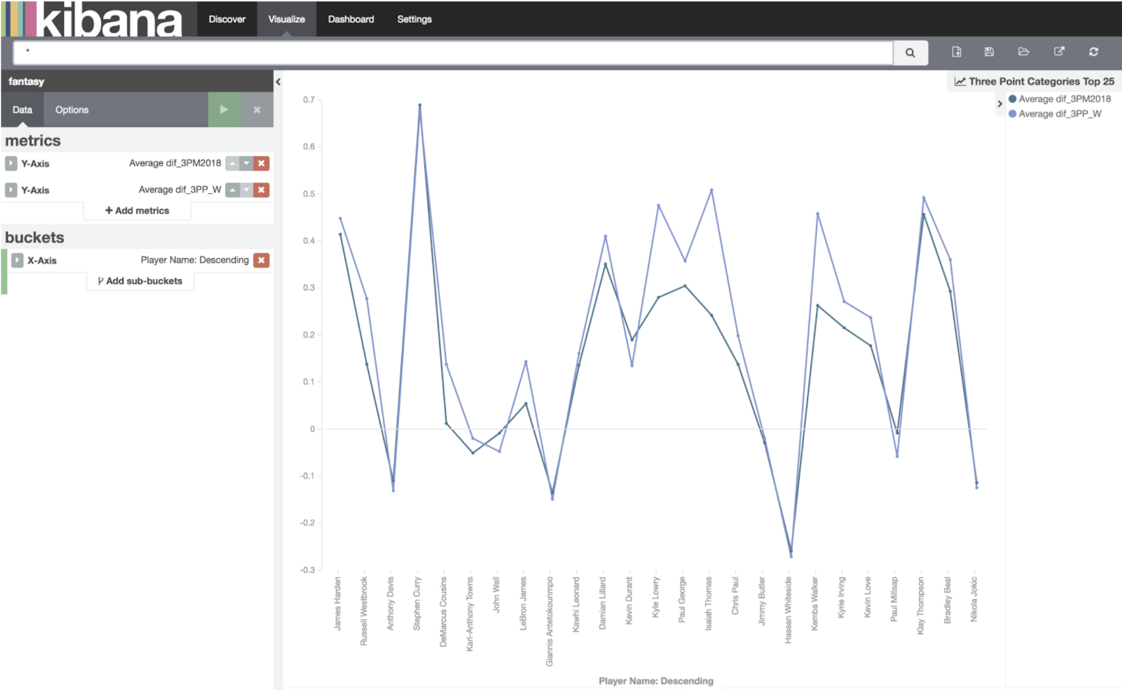
Three Point Categories Top 255
Applying the statistic over the whole list of players showed us some good news. If we only graph dif_BLK, dif_AST, and dif_DD, then it shows there is value in the later rounds for Blocks, and Assists. These would be categories I would not be punting, because in order to compete in them, I didn’t need to have a high draft pick.
Taking a further investigation into DD’s, we can see that there is no real value in the later rounds in DD’s. I would either need to invest heavily in the first few rounds, ensuring that I would be capable of winning the category, or I should not invest at all. At this stage, I’m going to punt DD’s.
BLK AST DD
Taking a further investigation into DD’s, we can see that there is no real value in the later rounds in DD’s. I would either need to invest heavily in the first few rounds, ensuring that I would be capable of winning the category, or I should not invest at all. At this stage, I’m going to punt DD’s.
Strategy Time
OK – time for some data exploration.
What happens if I only determine a player value based on categories I want to win?
So I’m going to remove double doubles, and the three point categories. Lets see what happens when I rerun the code, removing 3pp, 3pm, and DD’s.
We do this by running CalculateValue.py and then enter the category names we are actually trying to win.
So let’s go with ‘python3 getValue.py -url “<Elasticsearch URL of your cluster>” -u “elasticsearch password” -p “elasticsearch password” -n player_value_punted -s dif_AST2018,dif_PTS2018,dif_REB2018,dif_STL2018,dif_TO2018,dif_BLK2018,dif_FGP_W,dif_FTP_W’
Then, again using kibana, we need to Refresh Elasticsearch Fields, and then visualise:
- Line Chart, the player value,
- Add a metric, the average player_value_punted
- both against the player’s name, and let’s sort it using the player_value
- Top 25, descending
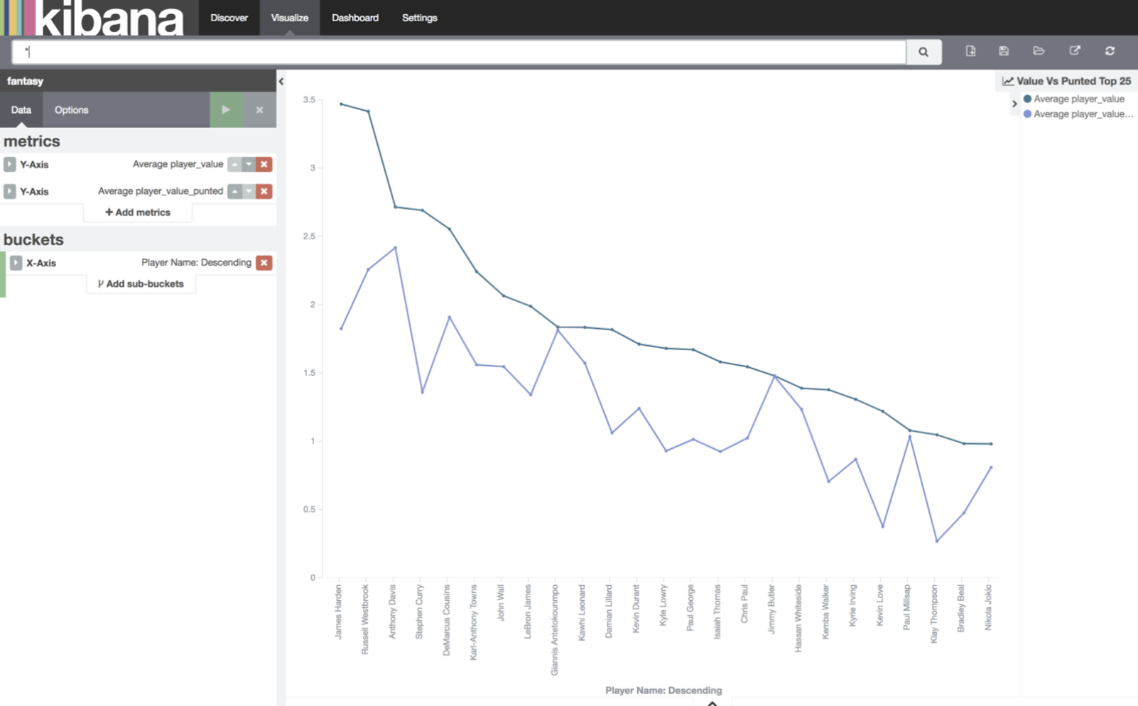
Value Vs Punted Top 25
You can see we have changed up the top 10 quite a bit, and if available, it shows who might be the best player for me to draft. Giannis Antetokounmpo. He is ranked #10 overall normally, but #4 when I apply my punted categories. The other player I should look to try and grab with the #14 pick: Jimmy Butler.
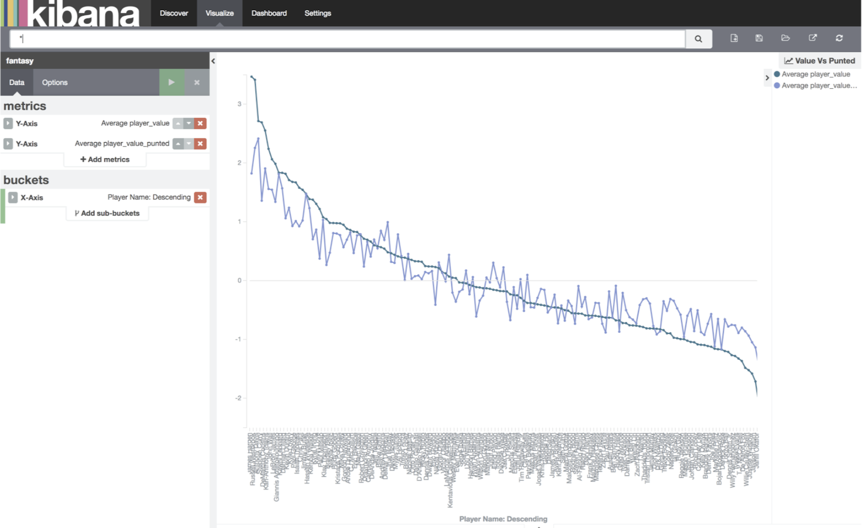
Value Vs Punted
Once we look deeper into the top 150, we can start to see the “peaks” of players who are going to be great value in my strategy: Giannis, Jimmy Butler, Myles Turner, Blake Griffin, DeMar Derozen, Jusuf Nurkic, Clint Capela, Ben Simmons. Players in the later rounds, are just going to be the best players I can get.
(Realistic) Dream Team
If I build my “Realistic Dream Team”, with players who are ranked around when I would be drafting, it would look a little something like this:
- #11 – Giannis Antetokounmpo(U)
- #14 – Jimmy Butler (SG)
- # 35 – Myles Turner (PF)
- # 37 – Blake Griffin (F)
- # 56 – DeMar Derozen (G)
- # 59 – Jusuf Nurkic (c)
- # 80 – Clint Capela (U)
- # 83 – Ben Simmons (PG)
- #104 – Rajon Rondo (G)
- # 107 – Nerlens Noel (U)
- #128 – Robin Lopez (B)
- # 131 – Josh Jackson (B)
- #152 – Markelle Fultz (B)
So how well would a team that looks like this perform?
Let’s have a look – Back to Kibana. Visualise:
- A bar chart, from a new search
- Plotting a sum of each of the categories
- Then, on the X axis, we are going to filter, and filter 1 will be each of the players names, separated by an “OR”.
- As you only play your top 10 players each week, I’m not going to include my last 3 draft picks in this graph.
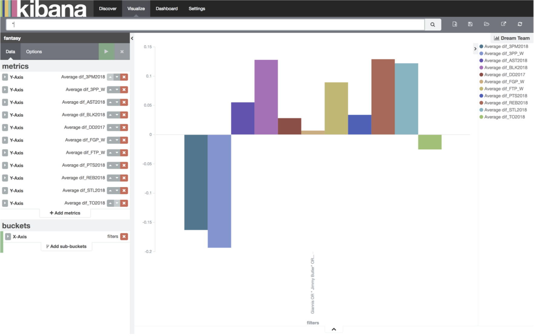
Dream Team
As we can see, this team will perform quite well. Above “average” in 8 of the 11 categories, and well above average in 4. The funny thing is, I was trying to punt DD’s, which it says I will do better than average, and lose TO’s, which I was trying to win.
Quick Comparison of Players
Now, this is the hard part.
Mike Tyson once said, “Everyone has a plan – until they get punched in the face”. On draft day, I can almost guarantee I won’t get my dream team. Someone will take a player I wanted, or I will need to change my strategy, on the fly. With 90 seconds to decide which player to draft, I need a way to quickly compare multiple possible players, quickly, on draft day.
Say someone nabs a player I want a couple picks before I can. I need a way to compare a couple players according to my punting strategy. Or say I need to swap my punting strategy on the fly, I can again use Kibana for this.
We go back to our ‘Categories with value’ line chart, and enter the player’s names in the filter – same as above.
Let’s have a look at an example, say, for argument’s sake I get the first four picks of my dream team. But DeMar DeRozen isn’t there at #5.
Who do I take?
Let’s say I’ve narrowed it down to Andrew Wiggins and Brook Lopez, and LaMarcus Aldridge. We can graph these three at a much more granular level. We go back to our earlier graph, and change it from Terms Player name, and change it to Filter. Then add a filter for each player.
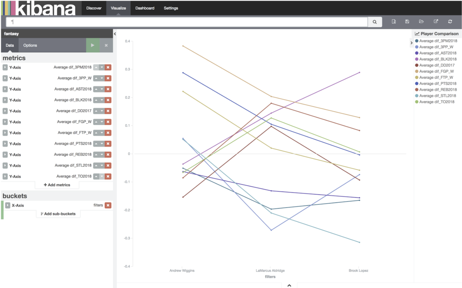
Player Comparison
This graph shows me that Andrew Wiggins is probably the best player to take, just because of his overall value. If I wanted to filter out categories which I was punting, I could just remove them.
Analysis on standby
So, with my dataset completed, and some queries ready to run come draft day, hopefully, I will be in the best position to draft the best players available
What else do I need before draft day?
Luck. A lot of good luck.