(Source: John Del Castillo)

Previously on the Machine Learning Series: 

This is the second article in our ongoing series exploring the machine learning landscape.  

In our previous article, we  

• Looked at the landscape of machine learning frameworks 
• Settled on using TensorFlow in Python for our maiden voyage 
• Set a goal for ourselves—to use the vast stream of metrics from Instaclustr’s Managed Service to make useful predictions and observations about the state of a cluster 
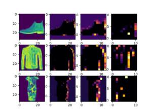
• And finally, worked through the first set of TensorFlow tutorials which focus largely on machine vision and convolutional neural networks (CNN).  

These tutorials gave us a great insight into how powerful this technology can be, but they don’t have much relevance to our desired goal. 

In this article, we’ll continue our adventure into machine learning with TensorFlow. 

What is a Neural Network? 

Before we dive into the practical work, we should understand the basics about what we are going to build—a neural network solution. 

A neural network is a type of machine learning solution which is designed to mimic the way a human brain operates. Multiple nodes, or neurons, are responsible for taking input from a problem, applying some sort of algorithm and then feeding the result to their interconnected neurons. 

This process repeats as many times as necessary until it achieves a result—a machine learning model that can be used to solve problems or make predictions. 

Choosing the Right Model 

In our previous article we worked through tutorials that employe CNN solutions, and I started to look at what other types of neural networks there were to find one that is appropriate for our goal of predicting cluster metrics. 

Unsurprisingly, there are a lot! From the basic perceptron and feed-forward networks all the way to deep convolutional and the newest flavor of the week, transformers. 

Mixed in there we can find the Recurrent Neural Network, or RNN, the description of which makes it a prime candidate for working with our metrics data 

“Recurrent neural networks (RNN) are a class of neural network that is powerful for modeling sequence data such as time series or natural language.”  Tensorflow.org 

The keyword in there being time series, like the metrics we want to analyze.  

And thus, we are drawn into a whole new set of tutorials and more reading to see how appropriate this technology is for our purposes. 

Additionally, all the models we’ve looked at until now have been classification models, where the algorithm will attempt to classify input with weighted probabilities, i.e., “this is a picture of a boot”.  

For our goals, we want something that can predict a value into the future based on data from the past. That is where we need to use a regression algorithm in our model. 

What Are Regression Algorithms? 

In simple terms, regression algorithms take sets of data as inputs and attempt to find relationships between a target value and the other values in the dataset. 

There are many types of regression algorithms, one being linear regression which attempts to plot a single line through the dataset and minimize the distance between the prediction and the datapoints. 

Machine learning frameworks support a wide variety of regression algorithms, and we can try multiple different algorithms to find the one most suited to the types of problem we are trying to solve. 

So now we have a solid idea of the type of model and the most appropriate technique, let’s see if we can find something to steer us in the right direction. 

Time Series Forecasting 

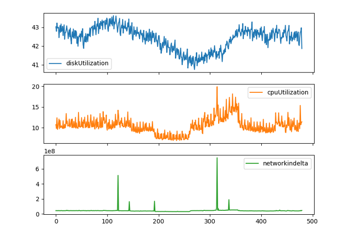
Visualization of metrics data set 

Once again, tensorflow.org has fantastic tutorials to help us navigate these waters. First, we can use the basic regression tutorial to get a feel for the problem we want to solve. 

This tutorial steps us through the process of training a model to use historical data, in this case engine specifications, to predict fuel efficiency. 

The approach is to expose the model to as much information as possible and allow it to make correlations between the various inputs and form a view on the world.  

Then, we introduce a new set of parameters, and ask the model to predict what it thinks the most likely value for fuel efficiency would be, and that is the general thrust of a how a regression model can work. 

Moving on to another tutorial, the time series forecasting tutorial goes even further into the process we need to get from data collection to model training. 

This tutorial uses a weather time series dataset recorded by the Max Planck Institute for Biogeochemistry. This dataset is incredibly detailed and is analogous to our own metrics data. 

The weather, specifically the temperature, changes slowly over time. This is like our disk usage metric we want to predict, which also changes slowly over time. 

In addition to helping us visualize the dataset, the tutorial also walks us through the process of cleaning the data and normalizing it. It also provides functions we can use to create data windows and batches which will allow us to build concurrency into the models we produce. 

It’s a terrific tutorial, which I highly recommend, and it is the perfect template for us to use for our own task. 

Defining Our Proof of Concept 

We have a fantastic template to follow, and now it’s time to start work and make something ourselves. 

The first iteration of our model is going to be a proof of concept with the following goal: 

Instaclustr stores metrics data for all our managed clusters in an Apache Cassandra® cluster. Most metrics are collected by node, every 20 seconds. This data can be queried by customers who want real-time metrics, but it’s short lived in our system with a Time to Live (TTL) of 2 weeks. 

We also process this data by rolling it up into 5 minute, hourly, and daily batches, where we summarize the data values. This data is longer lived and can be used to look further back in time and will be the source of our model data. 

The data is stored in our metrics cluster, known internally as Instametrics which is hosted exactly the same as a customer cluster in the Instaclustr Managed Service.  

Because this cluster is provisioned in our managed service, it also generates metrics about itself and sends them through the pipeline which ultimately stores the metrics back in itself. It stores metrics about its own nodes—confusing! 

Here is a diagram to help illustrate the metrics collection process: 

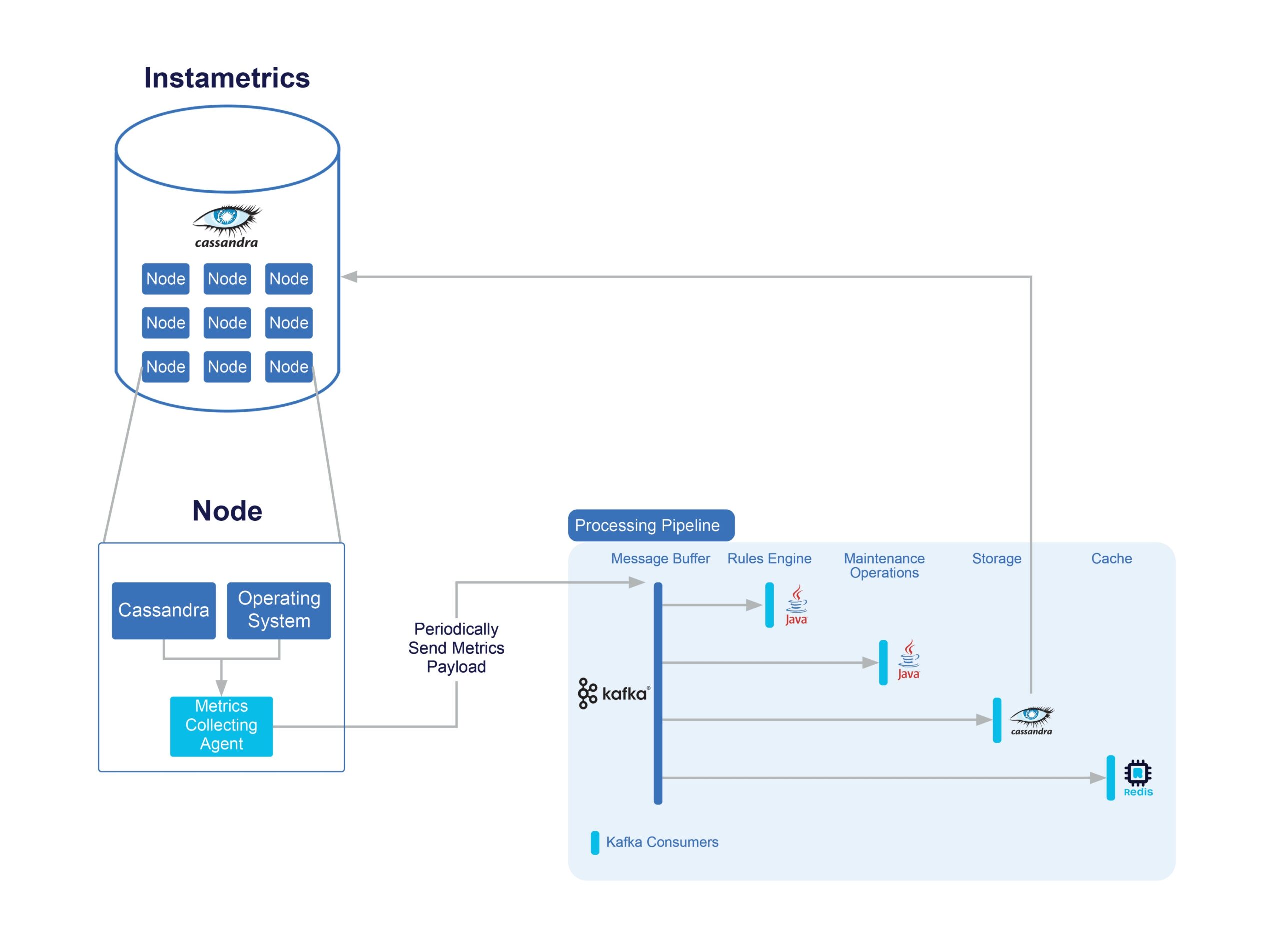
The Instametrics cluster provides the data which powers our automated monitoring systems, Technical Operations support tasks, and is also made available to our customers through our Monitoring API.

Our Monitoring API is documented here. The API has many options, but a call to it looks like this: 

We can query up to 20 different metrics, define a period which can range between the last 1 minute (1m), to the last 30 days (30d), and finally the end which is a timestamp for the final metric in the requested period. 

Using this API, I’ll be generating a dataset containing the last year of data for the Instametrics cluster. We will then train a model and, hopefully, create something that can predict disk usage 1 month into the future. 

Curating the Data 

Before we can extract some data and transform it into a format we can process with TensorFlow, we need to determine what metrics we want in the dataset.  

This itself is a big and important task! You can have the most sophisticated set of tools in the world, but if you use bad data, you will get a bad result. 

So, what is good data? We don’t always know! Some metrics may inform others, but it’s not necessarily obvious.  

Incoming network traffic could be a good indicator of data size on disk, but maybe the customer is always writing to the same key. High CPU load could mean lots of data is being processed, or that a large number of clients are just reading the data. 

Ideally, we would include as many metrics as possible, and then have the model itself determine which ones are relevant and which aren’t, without it getting too noisy. 

For this proof of concept, we can select a smaller set of data. I’ll start with a limited set of metrics and make sure the model is flexible enough to accept a larger number in the future. 

After reviewing the available metrics for a Cassandra cluster in our monitoring API, I narrowed it down to the following set: 

• CPU utilization 
• Disk utilization 
• Reads 
• Writes 
• Compactions 
• Client request read 
• Client request write 
• Network in delta 
• Network out delta 
• TCP established 

Now we can make a request to retrieve the data from the API. As we mentioned before, the API supports periods of data between 5 minutes and 30 days. These options inform the API which “bucket” of metrics to query.  

If we select 30 days, the API will return a single value, per metric, for each day in that period.  

However, we want to get hourly data points, so we will instead ask for 7 days of data, which ensures we will get the resolution of data we want.  

In future iterations of this model we may determine that daily metrics are sufficient, but for now we want as much data as possible. 

We compose the API request, and the result looks like this: 

The API returns a set of results for each node in the cluster, and within each node is a collection of metrics and their values. 

We’ll be requesting data in weekly batches, starting from the current date and moving backwards in time until we have around 1 year of hourly data for our cluster. 

This requires us to combine the data and convert it, and we’ll need to write a small application in Python to help us. 

Building the Data Collection Tool 

To keep things simple, we are going take just the data from the first node of our Cassandra cluster to make our dataset easier to understand.  

In our example above, this would be the first node of the JSON tree and we ultimately want to produce a CSV file which we can feed into our ML model.  

To achieve that, we take a 7-day set of metrics and convert it to a Python dictionary. After all the metrics are loaded in, we will then add it to a pandas dataframe, which allows us to append data to it by providing the dictionary.  

We’ll be using the same dataframe object in our model, but we want to save the data to disk first. 

The process continues and requests the next 7-day batch of data and keeps appending it until we finally save it to a CSV file. 

The Python code looks like this: 

After running the above program, I hit an issue where multiple keys had the same name in the payload response for a couple of metrics. This is due to them being Histogram metrics, which are themselves sets of metrics, including percentiles and others. 

For our task, we can just use the first set of values and ignore the rest, and after cleaning that up we had a CSV with all the metrics for a single Apache Cassandra node to use in our machine learning model, in chronological order. 

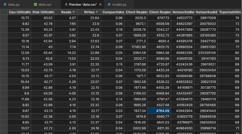
This data looks great! And it took longer than it should have to get it right! 

As a Python novice, it took a bit of trial and error to get the right values into the right data types. This is tricky because everything in Python is anything—until it isn’t! The method for building a Python application is different to that of Java or C# and it took me a while to adapt. 

Whatever doesn’t kill you will make you stronger, they say! So onwards we go. 

Moving on to Our Machine Learning Model 

In this article we investigated the various machine learning models that exist and identified the type of model we wanted to create for our task. We then found a tutorial that can serve as a template to build upon. 

We moved on and identified the data we will use to train our model and built a tool to collect and persist it. 

Join me in the next article, when we take this dataset, build a machine learning model, and finally see how successful we are at predicting the disk usage of a Cassandra cluster.