A Comprehensive Guide to Apache Cassandra Architecture

Introduction

Apache Cassandra architecture is designed to provide scalability, availability, and reliability to store massive amounts of data. If you are new to Cassandra, we recommend going through the high-level concepts covered in what is Cassandra before diving into the architecture.  

This blog post aims to cover all the architecture components of Cassandra. After reading the post, you will have a basic understanding of the components. This can be used as a basis to learn about the Cassandra Data Model, to design your own Cassandra cluster, or simply for Cassandra knowledge.

Editor’s note: Updated to reflect Apache Cassandra version 5.

This is part of a series of articles about Apache Cassandra.

What’s new in Apache Cassandra 5?

Apache Cassandra 5.0 is a landmark update that significantly expands the database’s functionality, performance, and ease of use. This release introduces advanced indexing and search capabilities, storage and memory improvements, expanded query language functions, and better operational tooling.

Key new features in Apache Cassandra 5.0

• Storage attached indexes (SAI): Cassandra now includes a modern secondary indexing mechanism that provides efficient and scalable queries on non-primary key columns, overcoming limitations of older index approaches and improving query performance across large datasets.
• Trie data structures for memtables and SSTables: New trie-based storage formats improve how data is organized both in memory and on disk, resulting in faster reads, faster writes, reduced memory overhead, and better performance for large datasets.
• Native vector data type and vector search: Cassandra 5.0 introduces support for vector data types and vector similarity search — a major step toward supporting AI and machine learning workflows directly in the database using high-dimensional embeddings.
• Unified Compaction Strategy (UCS): This new compaction engine simplifies data organization by dynamically adapting compaction policies, lowering operational overhead, and improving performance without manual tuning.
• Expanded CQL functions: New built-in mathematical functions (e.g., abs, exp, log, log10, round) enhance Cassandra Query Language (CQL) capabilities, enabling more complex computations directly in queries.
• JDK 17 support: Upgrading the underlying Java version to JDK 17 brings performance gains, improved garbage collection, and better overall resource management for production clusters.
• Dynamic data masking: Improved security support now includes the ability to mask sensitive fields in query results, helping with privacy and compliance requirements.
• New operational tooling: Cassandra 5.0 adds tools such as offline analysis utilities (e.g., for finding large partitions), a virtual system logs table for easier monitoring, and new authorizers (like CIDR rules) for flexible access control.
• Other enhancements: This release also includes TTL and writetime support on collections and user-defined types (UDTs), various guardrails to prevent risky operations, and improved guardrails and performance optimizations throughout the engine.

Cluster topology and design

Cassandra is based on distributed system architecture. In its simplest form, Cassandra can be installed on a single machine or in a docker container, and it works well for basic testing. A single Cassandra instance is called a node. Cassandra supports horizontal scalability achieved by adding more than one node as a part of a Cassandra cluster. The scalability works with linear performance improvement if the resources are configured optimally.

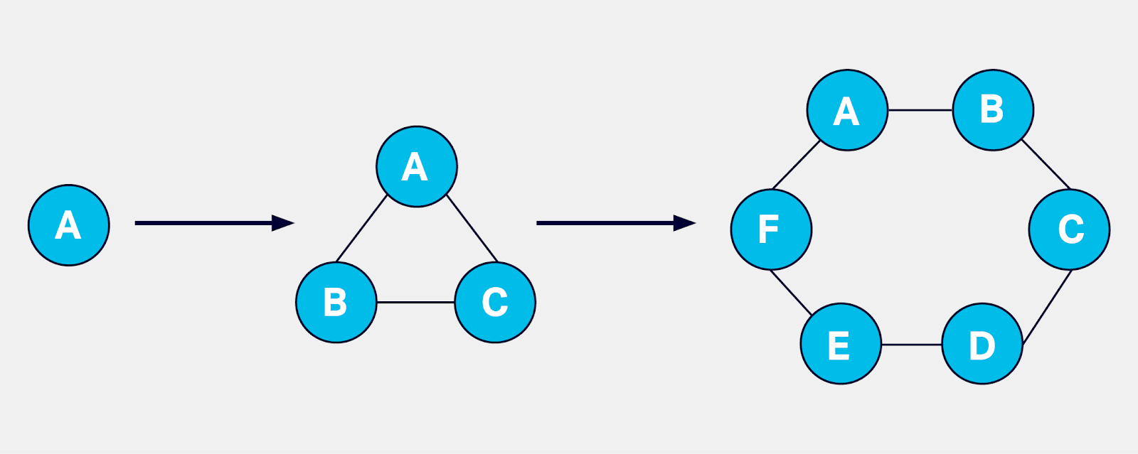
Cassandra works with peer to peer architecture, with each node connected to all other nodes. Each Cassandra node performs all database operations and can serve client requests without the need for a master node. A Cassandra cluster does not have a single point of failure as a result of the peer-to-peer distributed architecture. 

Nodes in a cluster communicate with each other for various purposes. There are various components used in this process:

• Seeds: Each node configures a list of seeds which is simply a list of other nodes. A seed node is used to bootstrap a node when it is first joining a cluster. A seed does not have any other specific purpose, and it is not a single point of failure. A node does not require a seed on subsequent restarts after bootstrap. It is recommended to use two to three seed nodes per Cassandra data center (data centers are explained below), and keep the seeds list uniform across all the nodes. 
• Gossip: Gossip is the protocol used by Cassandra nodes for peer-to-peer communication. The gossip informs a node about the state of all other nodes. A node performs gossip with up to three other nodes every second. The gossip messages follow specific format and version numbers to make efficient communication.

A cluster is subdivided into racks and data centers. These terminologies are Cassandra’s representation of a real-world rack and data center. A physical rack is a group of bare-metal servers sharing resources like a network switch, power supply etc. In Cassandra, the nodes can be grouped in racks and data centers with snitch configuration. Ideally, the node placement should follow the node placement in actual data centers and racks. Data replication and placement depends on the rack and data center configuration. 

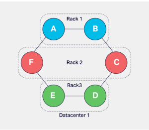
A rack in Cassandra is used to hold a complete replica of data if there are enough replicas, and the configuration uses NetworkTopologyStrategy, which is explained later. This configuration allows Cassandra to survive a rack failure without losing a significant level of replication to perform optimally. 

There are various scenarios to use multiple data centers in Cassandra. Few common scenarios are:

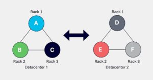
• Build a Cassandra cluster with geographically distinct data centers which cater to clients from distinct locations, e.g.a cluster with three data centers in US, EU, and APAC serving local clients with low latency.
• Separate Cassandra data centers which cater to distinct workloads using the same data, e.g. separate data centers to serve client requests and to run analytics jobs.
• Active disaster recovery by creating geographically distinct data centers, e.g. a cluster with data centers in each US AWS region to support disaster recovery.

Read more: Connecting to a Cassandra cluster using TLS/SSL

Database structures

Cassandra stores data in tables where each table is organized in rows and columns the same as any other database. Cassandra table was formerly referred to as column family. Tables are grouped in keyspaces. A keyspace could be used to group tables serving a similar purpose from a business perspective like all transactional tables, metadata tables, use information tables etc. Data replication is configured per keyspace in terms of replication factor per data center and the replication strategy.  See the replication section for more details.

Each table has a defined primary key. The primary key is divided into partition key and clustering columns. The clustering columns are optional. There is no uniqueness constraint for any of the keys.

The partition key is used by Cassandra to index the data. All rows which share a common partition key make a single data partition which is the basic unit of data partitioning, storage, and retrieval in Cassandra.  

Refer to Cassandra-data-partitioning for detailed information about this topic. 

Partitioning

A partition key is converted to a token by a partitioner. There are various partitioner options available in Cassandra out of which Murmur3Partitioner is used by default. The tokens are signed integer values between -2^63 to +2^63-1, and this range is referred to as token range. Each Cassandra node owns a portion of this range and it primarily owns data corresponding to the range. A token is used to precisely locate the data among the nodes and on the data storage of the corresponding node.  

It is evident that when there is only one node in a cluster, it owns the complete token range. As more nodes are added, the token range ownership is split between the nodes, and each node is aware of the range of all the other nodes. 

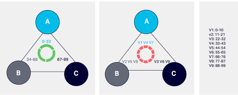
Here is a simplified example to illustrate the token range assignment. If we consider there are only 100 tokens used for a Cassandra cluster with three nodes. Each node is assigned approximately 33 tokens like: 

 node1: 0-33 node2: 34-66 node3: 67-99. 

 If there are nodes added or removed, the token range distribution should be shuffled to suit the new topology. This process takes a lot of calculation and configuration change for each cluster operation. 

Related content: Learn more about data architecture principles

Virtual nodes/Vnodes

To simplify the token calculation complexity and other token assignment difficulties, Cassandra uses the concept of virtual nodes referred to as Vnodes. A cluster is divided into a large number of virtual nodes for token assignment. Each physical node is assigned an equal number of virtual nodes. In our previous example, if each node is assigned three Vnodes and each Vnode 11 tokens: 

 v1:0-9, v2:10-19, v3:20-29 so on 

 Each physical node is assigned these vnodes as:

 node1: v1, v4, v7 node2: v2, v5, v8 node3: v3, v6, v9 

The default number of Vnodes owned by a node in Cassandra is 256, which is set by  num_tokens property. When a node is added into a cluster, the token allocation algorithm allocates tokens to the node. The algorithm selects random token values to ensure uniform distribution. But, the num_tokens property can be changed to achieve uniform data distribution. The number of 256 Vnodes per physical node is calculated to achieve uniform data distribution for clusters of any size and with any replication factor. In some large clusters, the 256 Vnode do not perform well please refer to blog cassandra-vnodes-how-many-should-i-use for more information.

Related content: Learn more in our detailed guide to Apache Cassandra on AWS

Replication

The data in each keyspace is replicated with a replication factor. The most common replication factor used is three. There is one primary replica of data that resides with the token owner node as explained in the data partitioning section. The remainder of replicas is placed by Cassandra on specific nodes using the replica placement strategy. All replicas are equally important for all database operations except for a few cluster mutation operations.

There are two settings that mainly impact replica placement. First is snitch, which determines the data center, and the rack a Cassandra node belongs to, and it is set at the node level. They inform Cassandra about the network topology so that requests are routed efficiently and allow Cassandra to distribute replicas by grouping machines into data centers and racks. GossipingPropertyFileSnitch is the goto snitch for any cluster deployment. It uses a configuration file called Cassandra-rackdc.properties on each node. It contains the rack and data center name which hosts the node. There is cloud-specific snitch available for AWS and GCP. 

The second setting is the replication strategy. The replication strategy is set at the keyspace level. There are two strategies: SimpleStrategy and NetworkTopologyStrategy. The SimpleStrategy does not consider racks and multiple data centers. It places data replicas on nodes sequentially. The NetworkTopologyStrategy is rack aware and data center aware. SimpleStrategy should be only used for temporary and small cluster deployments, for all other clusters NetworkTopologyStrategy is highly recommended. A keyspace definition when used with NetworkTopologyStrategy specifies the number of replicas per data center as:

Here, the keyspace named ks is replicated in dc_1 with factor three and in dc_2 with factor one.

Consistency and availability

Each distributed system works on the principle of the CAP theorem. The CAP theorem states that any distributed system can strongly deliver any two out of the three properties: Consistency, Availability and Partition-tolerance. Cassandra provides flexibility for choosing between consistency and availability while querying data. In other words, data can be highly available with a low consistency guarantee, or it can be highly consistent with lower availability. For example, if there are three data replicas, a query reading or writing data can ask for acknowledgments from one, two, or all three replicas to mark the completion of the request. For a read request, Cassandra requests the data from the required number of replicas and compares their write-timestamp. The replica with the latest write-timestamp is considered to be the correct version of the data. Hence, the more replicas involved in a read operation adds to the data consistency guarantee. For write requests, the requested number is considered for replicas acknowledging the write. 

Naturally, the time required to get the acknowledgement from replicas is directly proportional to the number of replicas requests for acknowledgement. Hence, consistency and availability are exchangeable. The concept of requesting a certain number of acknowledgements is called tunable consistency and it can be applied at the individual query level. 

There are a few considerations related to data availability and consistency: 

• The replication factor should ideally be an odd number. The common replication factor used is three, which provides a balance between replication overhead, data distribution, and consistency for most workloads.    
• The number of racks in a data center should be in multiples of the replication factor. The common number used for nodes is in multiples of three. 
• There are various terms used to refer to the consistency levels – 
  • One, two, three: Specified number of replicas must acknowledge the operation.
  • Quorum: The strict majority of nodes is called a quorum. The majority is one more than half of the nodes. This consistency level ensures that most of the replicas confirm the operation without having to wait for all replicas. It balances the operation efficiency and good consistency. e.g.Quorum for a replication factor of three is (3/2)+1=2; For replication factor five it is (5/2)+1=3.
  • Local_*: This is a consistency level for a local data center in a multi-data center cluster. A local data center is where the client is connected to a coordinator node. The * takes a value of any specific number specified above or quorum, e.g. local_three, local_quorum. 
  • Each_*: This level is also related to multi data center setup. It denotes the consistency to be achieved in each of the data centers independently, e.g. each_quorum means quorum consistency in each data center. 

The data written and read at a low consistency level does not mean it misses the advantage of replication. The data is kept consistent across all replicas by Cassandra, but it happens in the background. This concept is referred to as eventual consistency. In the three replica example, if a user queries data at consistency level one, the query will be acknowledged when the read/write happens for a single replica. In the case of a read operation, this could mean relying on a single data replica as a source of truth for the data. In case of a write operation, the remainder replicas receive the data later on and are made consistent eventually. In case of failure of replication, the replicas might not get the data. Cassandra handles replication shortcomings with a mechanism called anti-entropy which is covered later in the post. 

Related content: Learn more in our detailed Apache Cassandra tutorial

Query interface

Apache Cassandra uses Cassandra Query Language (CQL) as its primary interface for interacting with the database. CQL’s syntax is designed to resemble SQL, making it familiar to developers coming from relational systems, but it is tailored to Cassandra’s distributed, wide-column data model and does not support relational constructs like joins or arbitrary subqueries.

Through CQL, users define and manipulate schema objects such as keyspaces (namespaces for tables and replication settings) and tables, and perform data operations (inserts, updates, deletes, and selects) either via the interactive shell cqlsh or through client drivers for languages such as Java, Python, or Node.js. Tools like cqlsh help developers quickly connect to a running Cassandra cluster and execute CQL statements directly against it.

Example of typical CQL interactions:

Data storage

Cassandra’s storage engine is built around a Log-Structured Merge-Tree (LSM-tree) design optimized for high write throughput and horizontal scalability. Incoming writes are first appended to a commit log on disk to guarantee durability so that, in case of a crash, acknowledged writes can be recovered. Simultaneously, the same write is applied to an in-memory structure called a memtable, which buffers recent updates in sorted order.

Once the memtable exceeds its configured size or threshold, it is flushed to disk as an immutable SSTable (Sorted String Table) file. Multiple SSTables can accumulate over time and are periodically consolidated through compaction to improve read performance and reclaim space. This architecture avoids in-place updates and favors sequential writes, which helps Cassandra sustain very high write performance even under heavy load.

Example view of the write storage lifecycle:

• A write arrives and is immediately recorded in the commit log for durability.
• The write is stored in the in-memory memtable, making it visible to reads before being persisted.
• When the memtable fills, it is flushed to disk as a new SSTable file.

This layered design (commit log → memtable → SSTable) ensures fast writes with durability and supports efficient read paths that query both memory and disk.

Write path

When a write request enters a Cassandra cluster, any node can act as the coordinator — there’s no master node. The coordinator receives the client mutation and determines which replica nodes should persist it based on the partition key, token ranges, and replication strategy. It then forwards the mutation to those replicas and waits for acknowledgements according to the chosen consistency level (e.g., ONE, QUORUM). This logic enables Cassandra to scale and remain highly available even if some replicas are slow or temporarily unreachable.

Inside each replica node, the write follows a highly optimized sequence to ensure durability and performance. First, the mutation is appended to the commit log, an append-only write-ahead log on disk that guarantees durability. Next, the same data is written into an in-memory Memtable.

Memtables are sorted in memory by partition key and make recent writes immediately visible to reads. When the Memtable reaches its threshold (size or time), it is flushed to disk as an immutable SSTable (Sorted String Table) file. SSTables are never updated in place; instead, new data produces new SSTables, and background compaction later merges them to keep read performance efficient and reclaim space. Hinted handoff may also be used to temporarily store writes for downed replicas so they can be synchronized later.

Anatomy of a write operation on a node:

• Coordinator selection: Any node receiving the write becomes coordinator and selects replicas.
• Commit log append: The data is logged on disk for durability.
• Memtable update: The write is stored in memory and sorted.
• SSTable flush: When full, Memtables are flushed to disk as SSTables.
• Replica acknowledgements: The coordinator waits per the consistency level before replying.

This design avoids blocking disk reads during writes and enables very high throughput even under heavy load.

Read Path

A read begins similarly with the client sending a request to any node, which becomes the coordinator. The coordinator identifies the replica nodes that own the requested partition key based on the token range and the partitioner, and contacts them with a read request. Tunable consistency determines how many replicas must respond before the read is considered successful.

On each replica, Cassandra uses several in-memory and on-disk structures to efficiently locate the requested data. First, it checks the Memtable (the in-memory buffer) to see if recent writes contain the partition. If so, those results are merged with on-disk data. For on-disk sources, Cassandra uses Bloom filters (probabilistic in-memory structures) to quickly determine which SSTables might contain the partition, reducing unnecessary disk reads. If caches are enabled, the row cache or partition key cache may speed up lookups by avoiding disk seeks.

When a partition key isn’t cached, Cassandra uses a partition summary and partition index to find the correct offset in SSTables. Once located, data is read from disk and merged across SSTables using per-row timestamps to produce the most recent version. As part of consistency upkeep, Cassandra may perform read repair in the background to synchronize out-of-date replicas.

Anatomy of a read operation on a node:

• Coordinator selection and replica contact: The coordinator locates replica nodes for the key.
• Memtable check: In-memory write buffer may satisfy the request immediately.
• Cache and filters: Row cache, partition key cache, and Bloom filters help narrow disk access.
• Index lookup: Partition summaries and indexes determine the exact SSTable offset.
• Data merge and return: Data from Memtable and SSTables are merged and returned.

This multi-stage read path balances performance and consistency, ensuring the latest data is returned even when spread across several SSTables on disk.

Conclusion

Cassandra architecture is uniquely designed to provide scalability, reliability, and performance. It is based on distributed system architecture and operates on the CAP theorem.  Cassandra’s unique architecture needs careful configuration and tuning. It is essential to understand the components in order to use Cassandra efficiently.

Contact us to get expert advice on managing and deploying Apache Cassandra.