pgvector similarity search: Basics, tutorial, and best practices
How does pgvector support similarity search?
pgvector is an open source extension for PostgreSQL. By integrating natively with PostgreSQL, it removes the need to use external vector databases or retrieval systems, simplifying architecture for applications that require similarity search and machine learning capabilities.
Pgvector enables efficient vector similarity search directly within a PostgreSQL database. It allows for the storage of high-dimensional vectors and the execution of various similarity metrics to find data points that are “closest” to a given query vector.
Key similarity search capabilities include:
- Vector storage: pgvector introduces a vector data type in PostgreSQL, allowing for the direct storage of numerical vectors representing embeddings of various data types (e.g., text, images, audio).
- Similarity metrics: It supports common distance metrics for similarity search, including: L2 Distance (Euclidean Distance): Measures the straight-line distance between two vectors. Represented by the
<->operator. - Inner product: Measures the magnitude and direction of two vectors. Represented by the
<#>operator (returns negative inner product, so multiply by -1 for the actual inner product). - Cosine distance: Measures the cosine of the angle between two vectors, indicating their directional similarity. Represented by the
<=>operator. Cosine similarity is calculated as 1 –cosine_distance. - Indexing for performance: pgvector supports indexing techniques like HNSW (Hierarchical Navigable Small Worlds) to accelerate approximate nearest neighbor (ANN) searches on large datasets, significantly improving query performance.
A bit of background: What Is similarity search?
Similarity search is a technique used to find items in a dataset that are most similar to a given query item. Unlike traditional exact-match searches, similarity search compares high-dimensional representations, such as image embeddings or text vectors, to identify results that are not only identical but contextually or semantically close. This is central to use cases like image recognition, recommendation systems, and natural language processing where relevance is derived from approximate resemblance, not just strict equality.
There are multiple approaches to implementing similarity search. These typically use distance metrics to measure closeness between vectors, with lower distances indicating greater similarity. Indexing schemes and algorithmic optimizations ensure that searches remain efficient, even with large datasets and vectors with hundreds or thousands of dimensions, enabling real-time or near-real-time querying for interactive applications.
Tips from the expert

Perry Clark
Professional Services Consultant
Perry Clark is a seasoned open source consultant with NetApp. Perry is passionate about delivering high-quality solutions and has a strong background in various open source technologies and methodologies, making him a valuable asset to any project.
In my experience, here are tips that can help you better optimize similarity search with pgvector for real-world ML workloads:
- Select the right embedding model: Use
all-MiniLM-L6-v2for efficient, pre-trained embeddings with a balance of speed and accuracy. Chunk large documents to fit within the model’s context window. - Boost query speed with vector indexes: Optimize similarity search by creating vector indexes, such as
ivfflator HNSW, depending on your data volume and performance requirements. These indexes significantly improve query performance for large datasets - Streamline ingestion and queries: Pre-compute and store embeddings during ingestion for faster retrieval. Use DAOs to simplify database operations and consider caching results for real-time applications.
Tutorial: Vector similarity search within Postgres with pgvector
This tutorial walks through the steps to perform vector similarity search using the pgvector extension in PostgreSQL. You’ll learn how to install pgvector, create tables with vector columns, insert and query high-dimensional data, and optimize search performance using indexing techniques like HNSW and ivfflat.
1. Install and enable pgvector
Pick an install method for your environment:
Linux/Mac:
- Build from source:
git clone --branch v ... && make && make install - Docker:
docker pull pgvector/pgvector:pg - Homebrew:
brew install pgvectorfor supported formulas - PGXN:
pgxn install vector APT/Yum/pkg/conda-forge, orPostgres.app(v15+ includes pgvector)
Windows:
- Build with MSVC
nmakein a Developer Command Prompt, or useDocker / conda-forge. - Enable the extension in your database (once per DB):
CREATE EXTENSION vector;
2. Create a table with vector columns
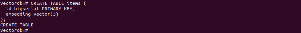
Use fixed dimensions when all vectors share the same size:
|
1 2 3 4 |
CREATE TABLE items ( id bigserial PRIMARY KEY, embedding vector(3) -- e.g., for 3-dim embeddings ); |
Or variable dimensions when sizes differ:
|
1 2 3 4 5 6 |
CREATE TABLE embeddings ( model_id bigint, item_id bigint, embedding vector, PRIMARY KEY (model_id, item_id) ); |
Note: Indexes can only cover rows with the same dimensionality when using variable-dim columns (use expression/partial indexes).
3. Load and modify data
Insert individual vectors:
|
1 2 |
INSERT INTO items (embedding) VALUES ('[1, 2, 3]'), ('[4, 5, 6]'); |

Bulk load with COPY (best with FORMAT BINARY). Example (Python/psycopg2 outline was provided in the source) writes vector bytes and uses copy_from to load into items(embedding).
Update and delete:
|
1 2 |
UPDATE items SET embedding = '[1, 2, 3]' WHERE id = 1; DELETE FROM items WHERE id = 1; |

4. Nearest-neighbor queries (exact scan)
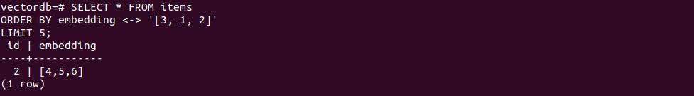
Order by a distance operator and limit results:
|
1 2 3 4 |
-- L2 (Euclidean) SELECT * FROM items ORDER BY embedding <-> '[3, 1, 2]' LIMIT 5; |
|
1 2 3 4 5 |
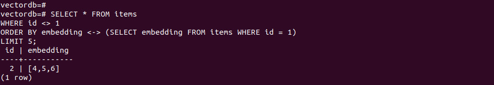
-- Compare to another row’s vector SELECT * FROM items WHERE id <> 1 ORDER BY embedding <-> (SELECT embedding FROM items WHERE id = 1) LIMIT 5; |
|
1 2 3 |
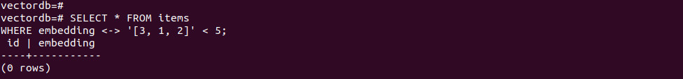
-- Distance filter SELECT * FROM items WHERE embedding <-> '[3, 1, 2]' < 5; |
Available operators:
<->L2 (Euclidean)<#>Inner product (returns negative inner product)<=>Cosine<+>L1 (Manhattan, pgvector ≥ 0.7.0)<~>Hamming (binary vectors, ≥ 0.7.0)<%>Jaccard (binary vectors, ≥ 0.7.0)
5. Distances and similarities
Compute distances/similarity:
|
1 2 |
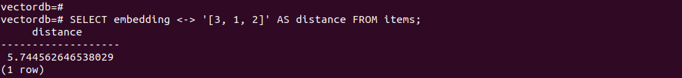
-- Return distances SELECT embedding <-> '[3, 1, 2]' AS distance FROM items; |
|
1 2 |
-- Cosine similarity = 1 - cosine_distance SELECT 1 - (embedding <=> '[3, 1, 2]') AS cosine_similarity FROM items; |

Aggregate vectors:
|
1 2 |
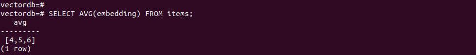
-- Mean vector SELECT AVG(embedding) FROM items; |

|
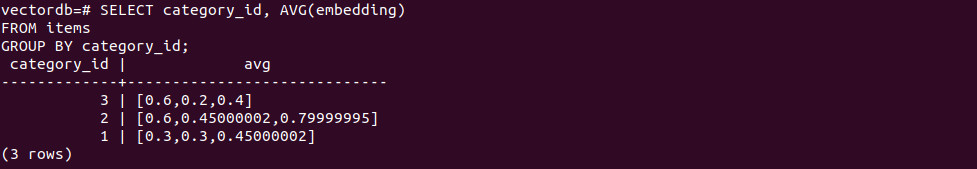
1 2 3 4 |
-- Mean per group SELECT category_id, AVG(embedding) FROM items GROUP BY category_id; |
6. Indexing for performance (ANN)
Exact vs. approximate
Exact gives perfect recall but is slow at scale; approximate (ANN) trades recall for speed.
HNSW
Create an HNSW index (pick the operator class for your metric):
|
1 2 3 4 5 6 |
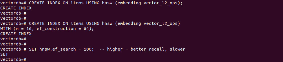
-- L2 example CREATE INDEX ON items USING hnsw (embedding vector_l2_ops); -- With build options CREATE INDEX ON items USING hnsw (embedding vector_l2_ops) WITH (m = 16, ef_construction = 64); |
Query-time control:
|
1 |
SET hnsw.ef_search = 100; -- higher = better recall, slower |
Tips: raise maintenance_work_mem and parallel workers to speed builds; monitor with pg_stat_progress_create_index.
Ivfflat
Partition vectors into lists (via k-means) and search selected lists:
|
1 2 3 |
-- L2 example with lists CREATE INDEX ON items USING ivfflat (embedding vector_l2_ops) WITH (lists = 100); |
|
1 2 |
-- Query-time probes (lists searched) SET ivfflat.probes = 10; -- higher = better recall, slower |

Guidance: choose lists ~ rows/1000 (≤1M rows) or ~√rows (>1M rows). Full-list probing is exact (planner won’t use the index).
7. Filtering with indexes
Add a standard index for post-filtering:
|
1 |
CREATE INDEX ON items (category_id); -- B-tree by default |
With ANN, filters run after the vector index scan. Increase hnsw.ef_search or ivfflat.probes to gather more candidates before filtering.
For few distinct filter values, use partial indexes:
|
1 2 |
CREATE INDEX ON items USING hnsw (embedding vector_l2_ops) WHERE (category_id = 123); |

For heavy filtering on one column, consider table partitioning.
Best practices for similarity search with pgvector
Here are some useful practices to consider when using pgvector for similarity search.
1. Optimize distance metrics for accuracy
The choice of distance metric directly affects search relevance. pgvector supports multiple metrics, each suited to different embedding characteristics:
- Cosine distance (
<=>): Suitable for text embeddings (e.g., BERT, Sentence Transformers) where the direction of vectors matters more than their magnitude. Cosine similarity ranges from -1 to 1 but is typically normalized between 0 and 1 when used in similarity search. - Euclidean distance (
<->): Works well when the absolute position of vectors in space carries meaning. Common in computer vision or structured feature vectors where the scale of each dimension is important. - Inner product (
<#>): Often used in ranking models or attention mechanisms where the dot product directly represents a scoring function. Can be converted to similarity by negating the result.
Selecting the wrong metric leads to poor search results. For example, applying Euclidean distance to unit-normalized text embeddings will penalize vectors with similar direction but different magnitudes, defeating the purpose of semantic similarity.
Before indexing, inspect your vector generation pipeline to verify whether vectors are normalized (unit vectors) and whether the training loss assumes a specific metric. Misaligned assumptions between embedding generation and retrieval reduce recall and precision in downstream tasks.
2. Balance exact and approximate search
Exact search evaluates the distance function against every row in the table. While it ensures optimal results, it becomes prohibitively slow as the dataset grows. For instance, a table with millions of vectors will result in millions of comparisons per query, regardless of hardware or index support.
Approximate nearest neighbor (ANN) search, on the other hand, uses indexing techniques (like HNSW or ivfflat) to dramatically reduce the search space. These indexes only evaluate a small, promising subset of candidates per query. However, the trade-off is that they may miss some close matches.
pgvector lets you tune recall vs. speed using:
ivfflat.probes: Higher values increase the number of lists searched, improving recall at the cost of latency.hnsw.ef_search: Similar effect; larger values mean more candidates considered during traversal.
Benchmark both modes under realistic query loads. For example, run precision@k and recall@k on a validation set, and measure query latency under concurrent load. Use exact search during development or evaluation, and switch to ANN with tuned parameters in production.
3. Choose between HNSW and Ivfflat
Both HNSW and ivfflat serve as ANN indexes, but their internals and behavior differ:
HNSW (hierarchical navigable small world):
- Graph-based structure; supports incremental inserts.
- Offers higher recall and lower query latency in large datasets.
- Tunable with
m(graph degree),ef_construction(index build quality), andef_search(query-time recall). - Suitable when query performance and accuracy are critical.
- Index build time is slower, and index size can grow large.
Ivfflat (inverted file index + flat quantization):
- Partitions data into k-means centroids (“lists”) and searches a fixed number of them.
- Requires pre-sorting vectors into lists during index creation.
- Faster to build and lower memory footprint.
- Tunable with
lists(index granularity) andprobes(search breadth). - More sensitive to the number of training vectors and can underperform if not tuned.
If your workload involves frequent vector inserts and updates, HNSW is more robust. For static datasets where you can afford to rebuild the index after batch inserts, ivfflat is lighter. Use real-world query benchmarks to make the final decision.
4. Hybrid and metadata-aware search
Most real-world applications require filtering based on metadata before or alongside vector similarity. For example, a recommendation engine might only show products in stock, in a certain category, or tailored to user demographics.
pgvector enables this with hybrid queries:
|
1 2 3 4 |
SELECT * FROM items WHERE category_id = 42 ORDER BY embedding <-> '[...]' LIMIT 10; |
However, ANN indexes (like ivfflat or HNSW) do not support filtering internally. PostgreSQL first performs the ANN scan and only then applies filters, which can reduce recall if the top-k set doesn’t include enough relevant results.
To mitigate this, increase ef_search (HNSW) or probes (ivfflat) to gather more candidates pre-filtering.
Use partial indexes to index only subsets of data with common filter values:
|
1 2 |
CREATE INDEX ON items USING hnsw (embedding vector_l2_ops) WHERE category_id = 42; |
For heavy filtering, partition tables by key columns (e.g., category), reducing the size of each index and query cost.
Designing queries that combine structured filters with vector search requires careful tuning to avoid recall loss while keeping latency low.
5. Watch out for non-indexable/ignored vectors
pgvector’s ANN indexes only apply to rows with vectors matching the dimensionality used at index creation. Any rows with mismatched dimensions, nulls, or empty vectors will be ignored during indexed queries.
For example, if you create an index on vector(768), rows with vectors of length 512 or NULL will not be part of the index scan and can lead to:
- Missed results (silent exclusion)
- Unexpected full table scans (when planner falls back to exact search)
- Confusing behavior in production
Best practices to avoid this:
- Use fixed-dimension vector types (e.g.,
vector(768)) whenever possible. - Validate incoming data to ensure all vectors conform to the required length.
Add CHECK constraints to enforce dimensionality:
|
1 2 |
ALTER TABLE items ADD CONSTRAINT check_vector_length CHECK (vector_dims(embedding) = 768); |
When using variable-length vectors, segment data using partial or expression indexes that only apply to rows with known valid dimensions.
This ensures consistency across inserts, prevents index misuse, and helps the planner make optimal decisions.
Harnessing AI with pgvector in PostgreSQL
Unlock powerful AI capabilities directly within your trusted PostgreSQL database using the pgvector extension, fully managed by Instaclustr. This combination transforms your data infrastructure into a dynamic engine for innovative applications, simplifying development while boosting performance. By integrating vector similarity search into PostgreSQL, you can build next-generation features without the complexity of managing a separate, specialized database. We make it easy to leverage your existing data and expertise to create truly intelligent solutions.
The core benefit for you is the ability to perform sophisticated vector similarity searches. The pgvector extension allows you to store and query high-dimensional vector embeddings—the numerical representations of unstructured data like text, images, or audio. This is the foundation of modern AI, enabling applications such as semantic search, personalized recommendation engines, and advanced fraud detection. Instead of bolting on another system, you can find the most relevant items in your dataset with remarkable speed and precision, all within the familiar PostgreSQL environment. This streamlined approach saves you time, reduces architectural complexity, and empowers your team to innovate faster.
Choosing Instaclustr’s managed PostgreSQL service amplifies these benefits. We take on the operational burden of database management, allowing you to concentrate on what matters most: building incredible applications. Our platform is engineered for exceptional reliability and effortless scalability, ensuring your database performance grows seamlessly with your AI workloads. With our 24/7 expert support and proactive monitoring, your PostgreSQL instances—supercharged with pgvector—are continuously optimized for peak performance. This gives you a secure, scalable, and worry-free foundation to confidently explore the full potential of AI.
For more information: