Massively Scalable Geospatial Anomaly Detection with Apache Kafka and Cassandra
After being Lost in (3D) Space in the last blog, in this final part of the geospatial anomaly detection series, we come back down to Earth and try out the Cassandra Lucene Plugin (this was our destination all along, but it’s a long way to Alpha Centauri!) We’ll also reveal how well a subset of the alternative solutions, from this and the previous 1-3 parts, actually worked.
1. The Cassandra Lucene Index
The Cassandra Lucene Index is a plugin for Apache Cassandra:
“… that extends its index functionality to provide near real-time search, including full-text search capabilities and free multivariable, geospatial and bitemporal search. It is achieved through an Apache Lucene based implementation of Cassandra secondary indexes, where each node of the cluster indexes its own data.
Recently we announced that Instaclustr is supporting the Cassandra Lucene Index plugin, and providing it as part of our managed Cassandra service. The full documentation for the plugin is here.
The documents say that “the plugin is not intended to replace Apache Cassandra denormalized tables, indexes, or secondary indexes, as it is just a tool to perform some kind of queries which are really hard to be addressed using Apache Cassandra out of the box features.”
Given that in the past 3 blogs we’ve investigated using all of these approaches to add geospatial queries to Cassandra, it’s finally time to take the Cassandra Lucene Index for a spin.
How does Lucene work? Lucene is built on a very ancient hand data mining technique which was originally used by Monks in 1230 to build a concordance of the Bible, it helped them find all the verses which had specific words in them (e.g. “Nephilim” – not many verses, “a” – lots of verses). A more recent (1890s) concordance was Strong’s “Exhaustive Concordance”, so-called not because it was heavy (it was, it weighed 3 KG making it bigger and heavier than the book it indexed, the Bible) but because it indexed every word, including “a”.
This is a good overview of Lucene (Lucene: The Good Parts), which helps make sense of this overview of the Lucene Cassandra plugin.
How is the Lucene Cassandra plugin used? It’s supported as an optional add-on in Instaclustr’s managed service offering, just select it in the Instaclustr Management Console when you are creating a Cassandra cluster and it is automatically deployed for you.
Lucene indexes are an extension of the Cassandra secondary indexes, so they are created using the CQL CREATE CUSTOM INDEX statement like this:
|
1 2 3 4 |
CREATE CUSTOM INDEX (IF NOT EXISTS)? <index_name> ON <table_name> () USING 'com.stratio.cassandra.lucene.Index' WITH OPTIONS = <options> |
To search using the index, this syntax is used.
|
1 |
SELECT * FROM test WHERE expr(<idx_name>, '<expr>'); |
Note that <options> and <expr> are JSON objects which actually specify what indexes are created and how they are searched. Also note that you only need to create a single Lucene index for each Cassandra table, as Lucene handles indexing all the requested columns for you.
Lucene indexes are queried using a custom JSON syntax defining the kind of search to be performed:
|
1 2 3 4 5 6 |
SELECT ( <fields> | * ) FROM <table_name> WHERE expr(<index_name>, '{ (filter: ( <filter> )* )? (, query: ( <query> )* )? (, sort: ( <sort> )* )? (, refresh: ( true | false ) )? }'); |
You can combine multiple filters, queries, and sorts (including sorting by geo distance). Note that queries are sent to all nodes in the Cassandra cluster. However, filters may find the results from a subset of the nodes, so filters will have better throughput than queries.
2. Geospatial Searches
How does this help for Geospatial queries? The Lucene plugin has very rich geospatial semantics including support for geo points, geo shapes, geo distance search, geo bounding box search, geo shape search, as well as multiple distance units, geo transformations, and complex geo shapes. We only need to use a subset of these for our geospatial anomaly detection use case.
The simplest concept is the geo point which is <latitude, longitude> coordinates. Interestingly, under the hood Indexing is done using a tree structure with geohashes (with configurable precision). Here’s how to create an index over latitude and longitude columns:
|
1 2 3 4 5 6 7 8 9 10 11 12 13 14 15 16 |
CREATE CUSTOM INDEX test_idx ON test() USING 'com.stratio.cassandra.lucene.Index' WITH OPTIONS = { 'refresh_seconds': '1', 'schema': '{ fields: { geo_point: { type: "geo_point", validated: true, latitude: "lat", longitude: "long", max_levels: 8 }' }; |
This index can be used to search for rows within a distance range from a specific point with this syntax:
|
1 2 3 4 5 6 7 8 9 10 |
SELECT ( <fields> | * ) FROM <table> WHERE expr(<index_name>, '{ (filter | query): { type: "geo_distance", field: <field_name> , latitude: <latitude> , longitude: <longitude> , max_distance: <max_distance> (, min_distance: <min_distance> )? }'); |
There’s also a bounding box search with syntax like this. Don’t forget you first have to convert distance to latitude and longitude for the bounding box corners:
|
1 2 3 4 5 6 7 8 9 10 |
SELECT ( <fields> | * ) FROM <table> WHERE expr(<index_name>, '{ (filter | query): { type: "geo_bbox", field: <field_name>, min_latitude: <min_latitude>, max_latitude: <max_latitude>, min_longitude: <min_longitude>, max_longitude: <max_longitude> }'); |
Partition-directed searches will be routed to a single partition, increasing performance. However, token range searches without filters over the partitioning column will be routed to all the partitions, with a slightly lower performance. This example fetches all nodes and all partitions so will be slower:
|
1 |
SELECT ( <fields> | * ) FROM <table> WHERE expr(<index_name>, '<expr>’); |
But this example fetches a single partition and will be faster:
|
1 |
SELECT ( <fields> | * ) FROM <table> WHERE expr(<index_name>, '<expr>’) AND <partition_key> = <value>; |
You can also limit the result set:
|
1 |
SELECT ( <fields> | * ) FROM <table> WHERE expr(<index_name>, '<expr>’) AND <partition_key> = <value> limit <limit>; |
Sorting is sophisticated, but note that you can’t use the CQL ORDER BY clause with the Lucene indexes. Here’s what the documentation says:
- When searching by filter, without any query or sort defined, then the results are returned in Cassandra’s natural order, which is defined by the partitioner and the column name comparator.
- When searching by query, results are returned sorted by descending relevance.
- Sort option is used to specify the order in which the indexed rows will be traversed.
- When simple_sort_field sorting is used, the query scoring is delayed.
Finally, prefix search is useful for searching larger areas over a single geohash column as you can search for a substring:
|
1 2 3 4 5 6 7 |
SELECT ( <fields> | * ) FROM <table> WHERE expr(<index_name>, '{ (filter | query): { type: "prefix", field: <field_name> , value: <value> }'); |
For example, to search for a 5 character geohash:
|
1 2 3 4 |
filter: { type: "prefix", field: "geohash", value: "every" |
Here are the Cassandra table and Lucene indexes we created to evaluate the performance:
|
1 2 3 4 5 6 7 8 9 10 11 12 13 14 15 16 17 18 19 20 21 22 |
CREATE TABLE latlong_lucene ( geohash1 text, value double, time timestamp, latitude double, longitude double, Primary key (geohash1, time) ) WITH CLUSTERING ORDER BY (time DESC); CREATE CUSTOM INDEX latlong_index ON latlong_lucene () USING 'com.stratio.cassandra.lucene.Index' WITH OPTIONS = { 'refresh_seconds': '1', 'schema': '{ fields: { geohash1: {type: "string"}, value: {type: "double"}, time: {type: "date", pattern: "yyyy/MM/dd HH:mm:ss.SSS"}, place: {type: "geo_point", latitude: "latitude", longitude: "longitude"} }' }; |
The simplest possible search is just using the partition key and a sort, Where <lat> and <long> are the location of the current event to check for an anomaly.
|
1 2 |
SELECT value FROM latlong_lucene WHERE expr(latlong_index, '{ sort: [ {field: "place", type: "geo_distance", latitude: " + <lat> + ", longitude: " + <long> + "}, {field: "time", reverse: true} ] }') and geohash1=<geohash> limit 50; |
The prefix search starts from geohash8 and increases the area until 50 rows are found:
|
1 |
SELECT value FROM latlong_lucene WHERE expr(latlong_index, '{ filter: [ {type: "prefix", field: "geohash1", value: <geohash>} ] }') limit 50 |
This query shows how the geo distance search works (distances are increased incrementally until 50 rows are found):
|
1 |
SELECT value FROM latlong_lucene WHERE expr(latlong_index, '{ filter: { type: "geo_distance", field: "place", latitude: " + <lat> + ", longitude: " + <long> + ", max_distance: " <distance> + "km" } }') and geohash1=' + <hash1> + ' limit 50; |
Finally, here’s the bounding box search, where the min and max bounding box latitudes and longitudes are computed based on increasing distance until 50 rows are found:
|
1 |
SELECT value FROM latlong_lucene WHERE expr(latlong_index, '{ filter: { type: "geo_bbox", field: "place", min_latitude: " + <minLat> + ", max_latitude: " + <maxLat> + ", min_longitude: " + <minLon> + ", max_longitude: " + <maxLon> + " }}') limit 50; |
3. And the Winner is …
 (Source: Shutterstock)
We tested a subset of the geospatial implementation alternatives we explored in this geospatial anomaly detection blog series, and ran throughput tests on identical Cassandra, Kafka and Kubernetes clusters to those we used in Anomalia Machina Blog 9.
Some high-level observations are that:
- There are many alternative ways of implementing geospatial proximity queries in Cassandra
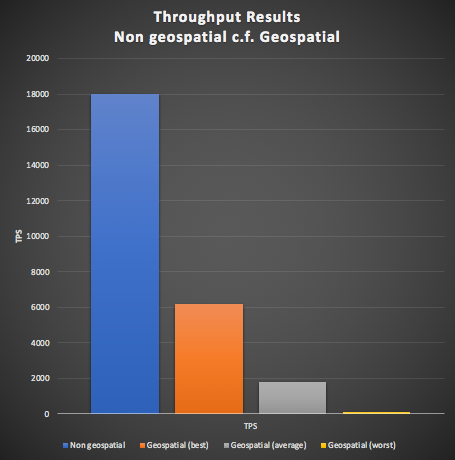
- The geospatial alternatives show significant variation (the graph below shows best, average and worst, the best geospatial results are 62 times better than the worst)
- The original non-geospatial results (18,000 TPS) are better than all the geospatial results, and
- The best geospatial results only achieve ⅓ the throughput of the original results, the average geospatial results are only 1/10th the original results.
However, this is not entirely unexpected, as the geospatial problem is a lot more demanding as (1) the queries are more complex being over 2 or 3 dimensions, and requiring calculation and of proximity between locations, and (2) more than one query is typically needed due to increasing the search area until 50 events are found.
Following are the detailed results. For some options, we tried both spatially uniform distributions of data, and dense data (clumped within 100km of a few locations), otherwise the default was a uniform distribution. We also tried a dynamic optimisation which kept track of the distance that returned 50 results and tried this distance first (which only works for uniform distributions).
3.1 Cassandra and Geohashes
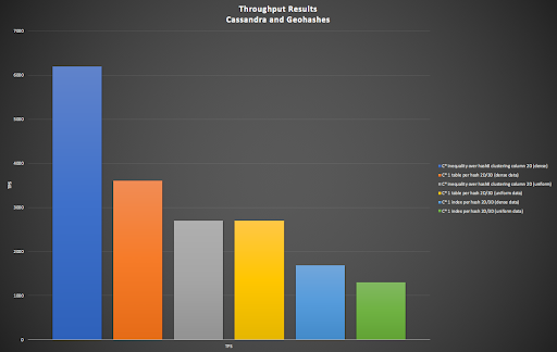
The following graph shows the results for the “pure” Cassandra implementations (Blog 2) including basic secondary indexes, all using geohashes. For most of the options both 2D and 3D geohashes are supported (Blog 3), with the exception of the option using “inequality over hash8 clustering column” which is 2D only (it relies on ordering which is not maintained for the 3D geohash). The results from worst to best are:
- Using 1 index for each geohash length 2D/3D (uniform, 1300 TPS, dense, 1690 TPS)
- 1 table for each geohash length 2D/3D (uniform, 2700 TPS), inequality over hash8 clustering column (2D only) (uniform, 2700 TPS)
- 1 table for each geohash length 2D/3D (dense, 3600 TPS)
- And the winner is, inequality over hash8 clustering column (2D only) (dense, 6200 TPS).
3.2 Cassandra Lucene Plugin/SASI and Latitude/Longitude
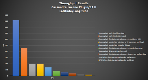
In this section, we evaluate the Cassandra Lucene Plugin (this blog) and SASI options (5.3). These options enabled the spatial searches over full latitude/longitude coordinates, using either bounding boxes or increasing distances. The exception was the Lucene prefix option (see above) which used a single geohash and the Lucene prefix operator to search shorter geohashes (and larger areas).
The most obvious thing to note is that the SASI options were the worst: SASI lat long clustering columns bounded box (dense, 100TPS, and uniform, 120TPS).
The Lucene options involved combinations of dense or uniform distributions, filtering by distance or bounding box, and sorted or not (in which case the client can sort the results). The results (from worst to best) were:
- filter by increasing distances, distance sort (uniform data, 200TPS)
- distance sort, no filter (uniform data, 300TPS)
- filter by increasing distances, no sort (uniform data, 400TPS)
- filter by bounded box increasing distance (700TPS)
- filter by bounded box, automatically optimised for most likely distance (1000TPS), equal with filter by increasing distances, no sort (dense data, 1000TPS)
- prefix filter (using geohashes, uniform data, 2300TPS, and with dense data 4600TPS).
Not surprisingly, the best result from this bunch used geohashes in conjunction with the prefix filter and Lucene indexes. There was not much to pick between the bounding box vs. distance filter options, with both achieving 1000 TPS (with distance optimisation or densely distributed data), probably because the geo point indexes use geohashes and both distance search types can take advantage of search optimisations using them.
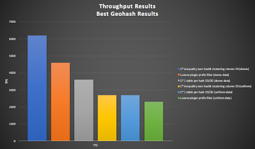
3.3 Best Geohash Results
The following graph shows the best six results (all using geohashes) from worst to best:
- The Lucene plugin prefix filter (uniform data, 2300 TPS) performed well, but was beaten by both the
- Cassandra 1 table per hash 2D/3D (uniform data, 2700 TPS) and Cassandra inequality over a single geohash8 clustering column 2D (uniform, 2700 TPS).
- The impact of assumptions around the data density are apparent as dense data reduces the number of queries required and increases the throughput dramatically with Cassandra 1 table per hash 2D/3D (dense data, 3600 TPS),
- and Lucene plugin prefix filter (dense data, 4600 TPS).
- And the overall winner is Cassandra inequality over a single geohash8 clustering column 2D (dense, 6200 TPS).
However, the worst and best results from this bunch are limited to 2D geospatial queries (but see below) whereas the rest all work just as well for 3D as 2D. The best result is the simplest implementation, using a single geohash as a clustering column.
Lucene options that use full latitude/longitude coordinates are all slower than geohash options. This is to be expected as the latitude/longitude spatial queries are more expensive, even with the Lucene indexing. There is, however, a tradeoff between the speed and approximation of geohashes, and the power but computational complexity of using latitude/longitude. For simple spatial proximity geohashes may be sufficient for some use cases. However, latitude/longitude has the advantage that spatial comparisons can be more precise and sophisticated, and can include arbitrary polygon shapes and checking if shapes overlap.
Finally, higher throughput can be achieved for any of the alternatives by adding more nodes to the Cassandra, Kafka and Kubernetes (worker nodes) clusters, which is easy with the Instaclustr managed Apache Cassandra and Kafka services.
4. “Drones Causing Worldwide Spike In UFO Sightings!”
If you really want to check for Drone proximity anomalies correctly, and not cause unnecessary panic in the general public by claiming to have found UFOs instead, then it is possible to use a more theoretically correct 3D version of geohashes. If the original 2D geohash algorithm is directly modified so that all three spatial coordinates (latitude, longitude, altitude), are used to encode a geohash, then geohash ordering is also ensured. Here’s example code in gist for a 3D geohash encoding which produces valid 3D geohashes for altitudes from 13km below sea level to geostationary satellite orbit. Note that it’s just sample code and only implements the encoding method, a complete implementation would also need a decoder and other helper functions.
The tradeoff between using the previous “2D geohash+rounded altitude” and this approach is that: (1) this approach is correct, but for the previous approach (2) the 2D part is still compatible with the original 2D geohashes (this 3D geohash is incompatible with it), and (3) the altitude is explicit in the geohash string (it’s encoded into and therefore only implicit in the 3D geohash).
 (Source: Shutterstock)
5. Conclusions and Further Information
In conclusion, using Geohashes with a Cassandra Clustering Column is the fastest approach for simple geospatial proximity searches, and also gives you the option of 3D for free, but Cassandra with the Lucene plugin may be more powerful for more complex use cases (but doesn’t support 3D). If the throughput is not sufficient a solution is to increase the cluster size.
The Instaclustr Managed Platform includes Apache Cassandra and Apache Kafka, and the (optional add-on) Cassandra Lucene Plugin can be selected at cluster creation and will be automatically provisioned along with Cassandra.
Try the Instaclustr Managed Platform with our Free Trial.