Welcome back to our ongoing series where I document a novice’s journey into the world of machine learning, mine. 

In our first article we started at the very basics of machine learning and investigated the various technologies and tutorials that exist out there. 

In Volume 2 we narrowed our search to find a machine learning model most appropriate for predicting values of time series data into the future. 

We then developed a program to collect data out of a REST API and collate it into a single table which we will now use to develop an ML model. 

Recurrent Neural Networks and Long Short-Term Memory 

In our previous article we decided that a recurrent neural network (RNN) sounded like the most appropriate model for our goal of predicting metrics, but we still need to explore what they are and how they work. 

Neural networks are designed to lightly mimic the way a human brain functions. They compromise a set of nodes—or neurons—that take the input data and apply weights and biases to them which then activate the downstream neurons in particular ways until we get to a final result. 

Recurrent neural networks build on this concept in a new way, where the results of previous operations are fed back into the neurons in a recurrent way.  

To contrast the two, a standard feed-forward network can be thought of as a path of steppingstones from Input to Output. By comparison, a recurrent neural network is more like a loop, that takes the input and uses it to further enhance the model until we achieve a result. 

Long short-term memory (LSTM) models are a further evolution of recurrent neural networks, which keep track of a “long term” memory in addition to processing short term information. The long-term memory is continually updated when the next value in the input data is processed until we reach the end of the processing chain and achieve our result. Pretty impressive stuff! 

Long short-term memory networks are a perfect place to start when making predictions with our time-series metrics data. 

Make Your Data Clean and Tidy  

We’ve collected our data and now we need to feed it to a machine learning model.  

As I mentioned in the previous article, we are using this Tensorflow tutorial as the basis for the model we’ll be developing. 

Using this guide, the first thing we should do is have a look at the data we’ve collected, and perform a sanity check on the fields. 

Let’s see the shape of the data for a few fields: 

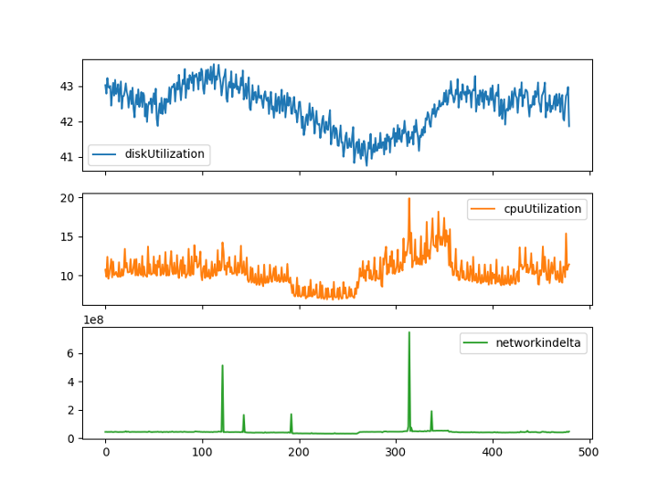
Looks like it passes the first test✅, there are no segments that appear out of order or suddenly shift wildly so I have confidence our data collector did everything correctly. 

Next up, let’s check for fields that may have values we can’t use or need to clean up. 

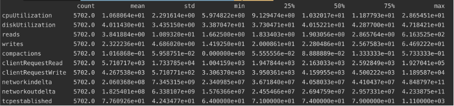
Another tick here ✅. There aren’t any null columns or values that are excessively outside the standard deviation. 

So, we have confidence our data is fit for purpose, so the final step is to normalize our data. 

Data normalization is a process where we standardize the scale for each column in our data. For example, in our data we have fields like disk and CPU utilization, which naturally have a scale between 0% and 100%, but another field like compactions has a different scale, generally between 0.05 to 0.1.  

Normalizing the data speeds up the machine learning process, allowing the algorithm to change the weights on each column in a consistent way and compare them more accurately to other column weights.  

Different machine learning algorithms may benefit more from data normalization techniques—in this example we are using data standardization, but your results may vary. For this example, I’m choosing normalization, but we can easily try the other if our result isn’t looking good. 

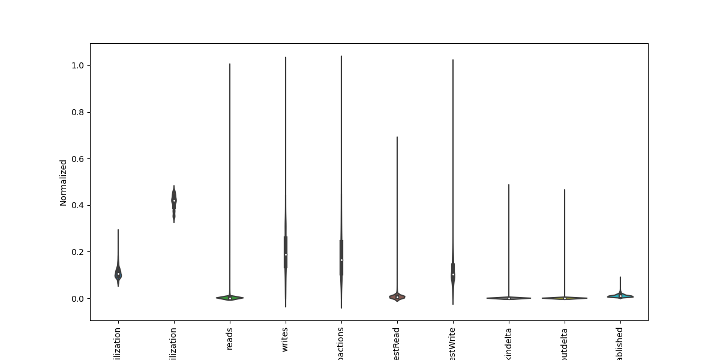
If we plot the distribution of our normalized data, we can see that some values are evenly distributed, and others are very lopped-sided—but this is the nature of our data. 

We also have two fields at the front, cpuUtilization and diskUtilization, which look different. The value of these fields is already a percentage, so there was no need to normalize the data, they are already naturally bounded at 0-100.  

All we did was divide them by 100 to get their values on the same scale. 

Here is the python code which normalizes our data: 

Data Splitting 

Ok we have prepared our data and identified our model, now we can start training it.  

For that, we need to provide 3 sets of data: train, validate, and test. We can do that by splitting the data we have into a 70-20-10 ratio.  

The training set is used by the model to tweak weights and biases in an iterative way until it has processed all the data and has settled on a particular view of the world. 

When the training is complete, the validation set is used to validate the accuracy of the produced model. We measure how far from reality the model is, and this result is then fed back into the next training iteration, or epoch, and the process continues. 

Importantly, the validation set isn’t used in the training of the model, only to validate it. 

Finally, the test set is used after the model is completely trained and validated. At this point, the model is as accurate as it can be given the parameters we’ve set, and we want to understand how accurate it is. 

We use the test set as a completely new batch of data and engage the model to measure its accuracy. 

Splitting our data introduces a problem. We have about 7 months of data, and we want to make predictions 1 month into the future. There isn’t enough data to split the data and train the model sufficiently. For that we need hundreds, or thousands, of sets, not 1. 

Visualizing our data, it looks like this: 

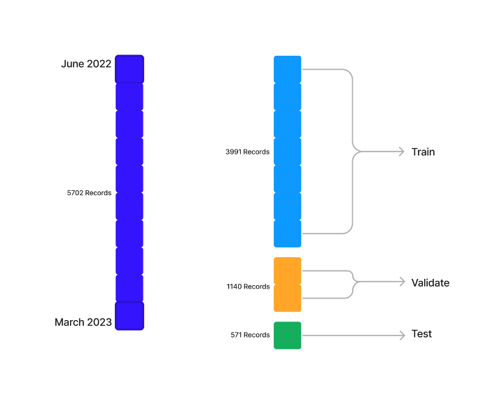
So, we need to make our first compromise. We need to reframe our goal to accommodate smaller data sets so we can train our model effectively. 

The challenge is that the value we are testing for, disk usage, changes much slower over short periods of time. If we don’t make our predictions far enough into the future, the model predictions will be comparable to just reusing the last known value. 

Luckily, we can squeeze the absolute maximum out of even the smallest data sets by using the timeseries_dataset_from_array function in Tensorflow. This allows us to create sliding windows over our data. 

Here is an example of how the sliding window works: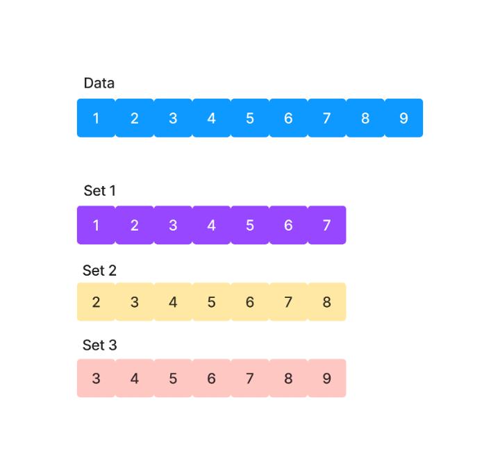 

The question is, what is the right size for our sets?

One benefit of being a complete novice is that I get to make uninformed decisions and see what happens!

I’m going to arbitrarily decide to split the test data into 32 data sets, which is the size of the batches we are creating. It makes sense that we have at least 1 batch in our test set.

The test set has 571 records in it, and because we can use the sliding window, the calculation looks like this

Each set will be 539 records wide, and as a reminder each record is a 1-hour time step. 

If we try to keep the same ratio, we were targeting originally of 7:1 (input data to prediction), we split that window into 471 hours of input and a prediction 67 hours into the future. 

Almost 3 days into the future, it’s a good start! 

Now all that’s left is to run the model and see how we went. 

Here is the code for the model, we are borrowing all of the heaper functions from our TensorFlow tutorial, and I’ll omit them here for brevity. 

Result Analysis 

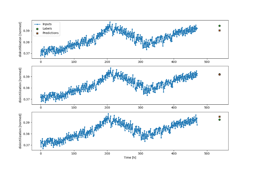
The results look pretty good! The above graph displays a sample of predictions taken from the training data. This is great but it’s the best possible scenario for the model and it is not a fair representation of how it will perform with unknown data.  

Still, it’s good to visualize how successful the model is with the training data it was provided with. It’s extremely accurate, the reported mean absolute error metric is 0.007, which is good!  

What does that value represent? The mean absolute error is how far off each prediction is, averaged out over the data set. Remember that disk utilization is a decimal value representing a percentage.  

So, this means, on average, the model predictions are within 0.7% of the actual value. If the target value is 10%, the model predicts a value between 9.3-10.7%.  

If we want to use these predictions to make decisions about cluster state for our Support teams, it is more than accurate enough. 

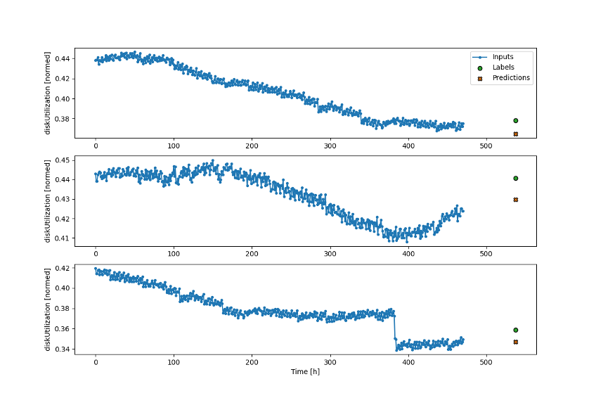
Moving on, we can now use our completed model with the test dataset and see how it goes with data it hasn’t seen before: 

It looks good!  

On closer inspection, it’s a little too good!  

We can look at the Y-axis and help explain why.  

This small data set operates in a very narrow range for our target data—between 37-39%. This means even if we selected a completely random point on this Y axis, we’d get within 2% of the actual value. 

It doesn’t necessarily mean the model is weak, but that our test data is a bit limited. 

To get a more meaningful test, we need more test data! 

The Final Assessment 

So how can we get more data that’s relevant to our test case? Luckily, I have a trick up my sleeve. 

Remember, we are using the Instaclustr monitoring API to build our dataset, and until now we’ve only been using the data from one node. But this particular cluster has over 70 nodes! 

I can re-use data.py which I used to create our csv file and modify it to format the data from another node. 

This is awesome because if your Cassandra cluster is well tuned, as ours is, the data usage and general load experienced by the cluster is evenly distributed across all the nodes. 

For our model, it means the trends and patterns that our model has learnt about diskUtilization are applicable for all other nodes in the cluster. 

With this new data in hand, the number of test windows grows from 32 to 220 and the data is much more varied, so it will really put our model to the test. 

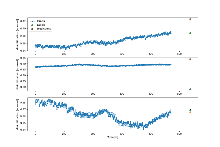
The results are good news, if not as good as the first attempt.  

Our mean absolute error on this dataset is 0.04, so on average the model is predicting the diskUtilization within 4% of the correct value. That result feels ok, although it could be better 

In the graphs, we can see in the second prediction that the model is making a pretty good guess, but the actual value suddenly dropped significantly.  

I feel like in an ideal world, whatever event caused this drop in disk utilization would be reflected in the metrics for the cluster and the model would be able to predict it closely, however in our case it looks like we aren’t including enough data to make this possible.  

Remember this is only our first attempt! As we improve our data sets and tune our model parameters, accuracy will likely improve. 

Finishing Up 

The goal of this series was to introduce myself to the world of machine learning and bring you along for the ride—and hopefully demonstrate what it takes to build a model using real world data. 

I am incredibly impressed with the maturity of Tensorflow and the quality of tutorials and guides that are out there to help people like me get started. 

The model we built is rudimentary, but it works and it’s clear that with a bit more dedication it could be developed into a full-fledged system.  

For Instaclustr, the possibilities are endless. We collect vast amounts of metrics, logs, and other data that we can start taking advantage of to develop machine learning systems that could deliver value to our customers who rely on us to run their business-critical applications in the cloud. 

In the future, we hope to be documenting these systems as they mature and are released, but for now I hope this series helped de-mystify a small part of the machine learning landscape for you and empowered you to start creating your own projects.