A Simple Classification Problem: Will the Monolith React? Is It Safe?!

Maybe a cautious approach to a bigger version of the Monolith (2km long) in a POD that is only 2m in diameter is advisable.   What do we know about how Monoliths react to stimuli? A simple classification problem consists of the category (label) “no reaction” (0) or “reaction” (1), and the stimuli tried (features which will be used to predict the label).  In the following table, the first column in the label to be predicted (positive, 1, or negative, 0), the remaining columns are the features, and each row is an example:

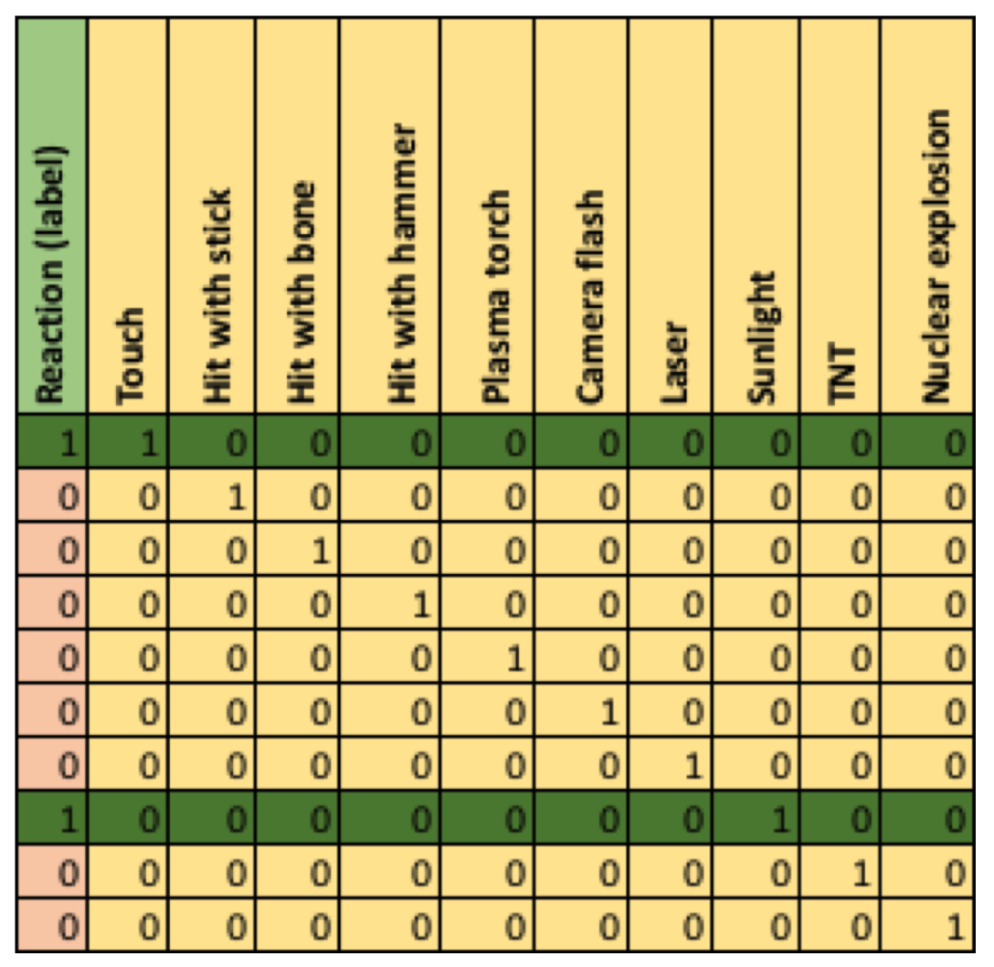
This problem is trivial as a positive reaction only occurred for Touch OR Sunlight (the camera flash was a coincidence), the features are all binary, and only a single feature at a time is true. As a result of extensive tests on the Monolith imagine that there are lots more examples and data available, each feature is a floating-point number, all features don’t have values for all examples, there are potentially 1,000s of features, and a sufficiently accurate classification rule may require an arbitrary number of features.

Given that HAL has been unplugged we have to analyze the data ourselves. What do we have available in the POD?

Apache SPARK and MLLib

One approach is to use an appropriately 1960’s-vintage machine learning algorithm suitable for simple binary classification problems. Decision tree algorithms were invented in the 1960’s (Concept Learning System, by a Psychologist, Earl Hunt), were improved in the 1980’s (e.g. ID3, C4.5, and FOIL, which references my 1988 machine learning algorithm, Gargantubrain), and are still useful. Spark’s Machine Learning Library (MLLib) has a number of regression and classification algorithms, including decision trees, that improve on the originals by running them “transparently” in parallel on multiple servers for scalability.

Spark’s scalable ML library is available here. It’s easy to download Spark and run MLLib examples locally, but the scalability benefits are best realised after deployment to an Instaclustr managed Spark cluster. Here’s the documentation on the MLLib decision tree algorithm.

Training

We’ll have a look at the example Java code, starting from the call to the decision tree algorithm to build the model from the examples, and working out from there. DecisionTree and DecisionTreeModel documents are relevant.  Here’s the code.  Note the API for trainClassifier:

trainClassifier(JavaRDD<LabeledPoint> input, int numClasses,
java.util.Map<Integer,Integer> categoricalFeaturesInfo, String
impurity, int maxDepth, int maxBins)

The first argument is a JavaRDD of LabeledPoint. The other arguments are for control of the algorithm:

// Set parameters for DecisionTree learning.

// Empty categoricalFeaturesInfo indicates all features are continuous.

Integer numClasses = 2;

Map<Integer, Integer> categoricalFeaturesInfo = new HashMap<>();

String impurity = “gini”; // or “entropy”

Integer maxDepth = 5;

Integer maxBins = 32;

// Train DecisionTree model

DecisionTreeModel model = DecisionTree.trainClassifier(trainingData, numClasses, categoricalFeaturesInfo, impurity, maxDepth, maxBins);

System.out.println(“Learned classification tree model:\n” + model.toDebugString());

What is a JavaRDD and LabeledPoint?

LabeledPoint

https://spark.apache.org/docs/latest/mllib-data-types.html#labeled-point

https://spark.apache.org/docs/latest/api/java/org/apache/spark/mllib/regression/LabeledPoint.html

Decision trees are a type of supervised learner, so we need a way of telling the algorithm what class (positive or negative for binary classifiers) each training example is.  LabeledPoint is a single labelled example (a “point” in n-dimensional space). It’s a tuple consisting of a Double label (either 0 or 1 for negative or positive examples), and a Vector of features, either dense or sparse.  Features are numbered from 0 to n. These are the examples from the documentation. Note the Vectors import. This is important as the default Spark Vector is NOT CORRECT.

import org.apache.spark.mllib.linalg.Vectors;
import org.apache.spark.mllib.regression.LabeledPoint;

// Create a labeled point with a positive label and a dense feature vector.

// There are three features, with values 1, 0, 3.
LabeledPoint pos = new LabeledPoint(1.0, Vectors.dense(1.0, 0.0, 3.0));

// Create a labeled point with a negative label and a sparse feature vector.

// There are two features, 0 and 2, with values 1 and 3 respectively.

LabeledPoint neg = new LabeledPoint(0.0, Vectors.sparse(3, new int[] {0, 2}, new double[] {1.0, 3.0}));

Resilient Distributed Datasets (RDDs)

https://spark.apache.org/docs/latest/rdd-programming-guide.html

https://spark.apache.org/docs/latest/api/java/org/apache/spark/api/java/JavaRDD.html

From the documentation:

“Spark revolves around the concept of a resilient distributed dataset (RDD), which is a fault-tolerant collection of elements that can be operated on in parallel. There are two ways to create RDDs: parallelizing an existing collection in your driver program or referencing a dataset in an external storage system… “ (such as Cassandra)

This blog has a good explanation of the Spark architecture, and explains that the features of RDDs are:

• Resilient, i.e. fault-tolerant with the help of RDD lineage graph and so able to recompute missing or damaged partitions due to node failures.
• Distributed with data residing on multiple nodes in a cluster.
• Dataset is a collection of partitioned data with primitive values or values of values, e.g. tuples or other objects (that represent records of the data you work with).

RDD’s are also immutable and can be cached. Fault-tolerance depends on the execution model which computes a Directed Acyclic Graph (DAG) of stages for each job, runs stages in optimal locations based on data location, shuffles data as required, and re-runs failed stages.

LIBSVM—Sparse Data Format

https://spark.apache.org/docs/2.0.2/mllib-data-types.html

https://spark.apache.org/docs/latest/api/java/org/apache/spark/mllib/util/MLUtils.html

Where does the RDD training data come from? In the example code I read it from a local file using MLUtils.loadLibSVMFile() (I’ll come back to the parameters later):

JavaRDD<LabeledPoint> data = MLUtils.loadLibSVMFile(sc, path).toJavaRDD();

From the documentation:

“It is very common in practice to have sparse training data. MLlib supports reading training examples stored in LIBSVM format, which is the default format used by LIBSVM and LIBLINEAR. It is a text format in which each line represents a labeled sparse feature vector using the following format:

label index1:value1 index2:value2 …

where the indices are one-based and in ascending order. After loading, the feature indices are converted to zero-based.”

For the above Monolith example the LIBSVM input file looks like this (assuming that feature values of “0” indicate non-existent data):

1.0 1:1.0
0.0 2:1.0
0.0 3:1.0
0.0 4:1.0
0.0 5:1.0
0.0 6:1.0
0.0 7:1.0
1.0 8:1.0
0.0 9:1.0
0.0 10:1.0

This doesn’t seem very “user friendly” as we have lost the feature names. I wonder if there is a better data format?

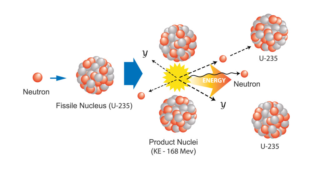
Splitting (the Data, Not the Atom)

(Source: Shutterstock)

Once we have the training data in the correct format for the algorithm (JavaRDD<LabeledPoint>), but before we train the model, we need to split it into two random subsets for training and testing. JavaRDD.randomSplit() does this and takes parameters:

double[] weights – weights for splits, will be normalized if they don’t sum to 1

long seed – random seed

// Split sample RDD into two sets, 60% training data, 40% testing data. 11 is a seed.

   JavaRDD<LabeledPoint>[] splits = data.randomSplit(new double[]{0.6, 0.4}, 11L);

   JavaRDD<LabeledPoint> trainingData = splits[0].cache();  // cache the data

   JavaRDD<LabeledPoint> testData = splits[1];

Notice the cache() call for trainingData.  What does it do? Spark is Lazy, it doesn’t evaluate RDD’s until an action forces it to. Hence RDD’s can be evaluated multiple times which is expensive. cache() creates an in memory cache “checkpoint” of an RDD which can be reused. The most obvious case is when an RDD is used multiple times (i.e. iteration), or for branching transformations (i.e. multiple different RDD’s are computed from an original RDD), in which case the original should be cached.
https://stackoverflow.com/questions/28981359/why-do-we-need-to-call-cache-or-persist-on-a-rdd

Note that for this example the initial data should be cached as we use it later to count the total, positive and negative examples.

Evaluating the Model on the Test Data – Thumbs down or up?

(Source: Shutterstock)

We trained a decision tree model above. What can we do with it? We trained it on the trainingData subset of examples leaving us with the testData to evaluate it on. MLLib computes some useful evaluation metrics which are documented here:

https://spark.apache.org/docs/latest/mllib-evaluation-metrics.html

https://spark.apache.org/docs/latest/api/java/org/apache/spark/mllib/evaluation/BinaryClassificationMetrics.html

Here’s the code which computes the evaluation metrics:

// Compute evaluation metrics.
BinaryClassificationMetrics metrics = new BinaryClassificationMetrics(predictionAndLabels.rdd());

The highlighted parameter is an RDD of (prediction, label) pairs for a subset of examples. I.e. (0, 0) (0, 1) (1, 0) (1, 0). I.e. for each example, run the model and return a tuple of predicted label and actual example label. Here’s the complete code that does this on the testData and then computes the evaluation metrics:

// For every example in testData, p, replace it by a Tuple of (predicted category, labelled category)

// E.g. (1.0,0.0) (0.0,0.0) (0.0,0.0) (0.0,1.0)

JavaPairRDD<Object, Object> predictionAndLabels = testData.mapToPair(p ->

    new Tuple2<>(model.predict(p.features()), p.label()));

// Compute evaluation metrics.

BinaryClassificationMetrics metrics = new BinaryClassificationMetrics(predictionAndLabels.rdd());

How does this work? There may be a few unfamiliar things in this code which we’ll explore: Tuple2, JavaPairRDD, mapToPair, features() and label().

Tuple(ware)

Java doesn’t have a built-in Tuple type, so you have to use the scala.Tuple2 class.

MAP

(Source: Shutterstock)

Map is an RDD transformation. Transformations pass each dataset element through a function and return a new RDD representing the result. Actions return a result after running a computation on a dataset. Transformations are lazy and are not computed until required by an action. In the above example, for every example in testData, p, it is replaced by a Tuple of (predicted category, labelled category). These values are computed by running model.predict() on all the features in the example, and using the label() of the example.

See LabeledPoint documentation for features() and label() methods.

JavaPairRDD is a (key, value) version of RDD. Instead of the general map function you need to use mapToPair.

Map (and mapToPair) are examples of “Higher Order Functions”. These are used a lot in Spark but are really pretty ancient and were first practically used in 1960 in LISP. Disturbingly the abstract sounds like an early attempt at HAL:

“A programming system called LISP … was designed to facilitate experiments … whereby a machine could be instructed to … exhibit “common sense” in carrying out its instructions.”

I used LISP for a real AI project (once), but (it ((had too) (many) brackets) (for (((me (Lots of Idiotic Spurious Parentheses))) ???!!! (are these balanced?!).

preferred(I, Prolog).

The following code prints out the main evaluation metrics, precision, recall and F.

JavaRDD<Tuple2<Object, Object>> precision = metrics.precisionByThreshold().toJavaRDD();

   System.out.println(“Precision by threshold: ” + precision.collect());

   JavaRDD<Tuple2<Object, Object>> recall = metrics.recallByThreshold().toJavaRDD();

   System.out.println(“Recall by threshold: ” + recall.collect());

   JavaRDD<Tuple2<Object, Object>> f = metrics.fMeasureByThreshold().toJavaRDD();

   System.out.println(“F by threshold: ” + f.collect());

Note that the metrics are designed for algorithms that can have multiple threshold values (i.e. the classification can have an associated probability).  However, the decision tree algorithm we are using is a simple yes/no binary classification.  A “confusion matrix” is a simple way of understanding the evaluation metrics. For each of the two states of reality (no reaction or reaction from the monolith) the model can make a true or false prediction giving four possible outcomes: Correct: TN = True Negative (the model correctly predicted no reaction), TP = True Positive (correctly predicted a reaction). And Incorrect: FP = False Positive (predicted a reaction but there was no reaction), FN = False Negative (predicted no reaction but there was a reaction).  FP is often called a Type I error, and FN a type II error.

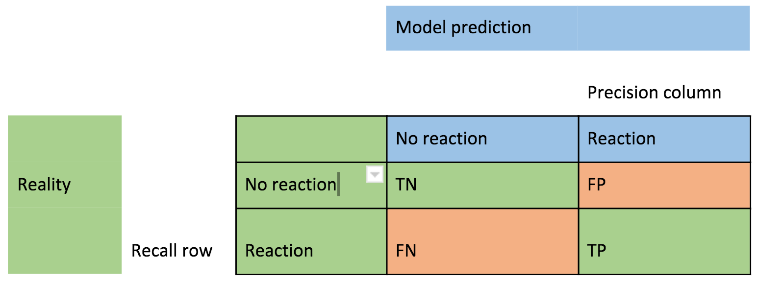
Precision = (TP)/(TP+FP), the proportion of predicted positives that were actually positive (the right column).

Recall = (TP)/(TP+FN), the proportion of actual positives that were correctly predicted as positive (the bottom row).

F is the average of precision and recall.

And the results (on the extended When Will the Monolith React? data) were as follows:

Precision = 71%

Recall = 45%

F = 56%

Precision is better than recall. 71% of the models predicted “Reaction” cases were in fact a “Reaction”. However, the model only correctly predicted 45% of all the actual “Reaction” cases correctly. The reason for using precision and recall metrics is to check if the model performance is purely the result of guessing. For example, if only 20% of examples are positive, then just guessing will result in a model “accuracy” approaching 80%.

FILTER

Another common Spark transformation is filter.   We’ll use filter to count the number of positive and negative examples in the data to check if our model is any better than guessing. filter() takes a function as the argument, applies it to each element in the dataset, and only returns the element if the function evaluates to true.

This code calculates that there are 884 examples, 155 positive and 729 negative, giving:

probability of positive example = 0.1753393665158371

probability of negative example = 0.8246606334841629

This tells us that just guessing would result in close to 82% accuracy. The actual model accuracy for the example is 85% (which requires extra code, not shown).

Spark Context

http://spark.apache.org/docs/latest/rdd-programming-guide.html

https://spark.apache.org/docs/latest/api/java/org/apache/spark/SparkContext.html

This leaves us with the final but “important bit” of the code at the start.  How is Spark actually run?  A SparkContext object tells Spark how to access a cluster, and a SparkConf has information about your application.  Given that we are just running Spark locally just pass “local” to setMaster.

SparkConf conf = new SparkConf().setAppName(“Java Decision Tree Classification Example”);
conf.setMaster(“local”);
SparkContext sc = new SparkContext(conf);
String path = “WillTheMonolithReact.txt”;

To run Spark on a cluster you need (a) a cluster with Spark set-up (e.g. an Instaclustr cluster with Spark add-on), and (b) to know more about the Spark architecture and how to package and submit applications.

How does this help with our approach to the Monolith? Maybe raising the POD’s manipulators in “greeting”? Will it be friends?

(Source: Shutterstock)

NOTE 1:

The actual data I used for this example was from the Instametrics example introduced in previous blogs, with the goal of predicting long JVM Garbage Collections in advance. I took a small sample of JVM-related metrics, and computed the min, avg and max for each 5 minute bucket. These became the features. For the label I determined if there was a long GC in the next 5 minute bucket (1) or not (0).  The real data has 1,000s of metrics, so next blog we’re going to need some serious Spark processing even just to produce the training data, and explore the interface to Cassandra, and the suitability of Cassandra for Sparse data.

NOTE 2:

Space travel is sooooo slow, in the years we’ve been on board Spark has changed from RDD to DataFrames. I’ll revise the code for the next blog.

Guide https://spark.apache.org/docs/latest/ml-guide.html

As of Spark 2.0, the RDD-based APIs in the spark.mllib package have entered maintenance mode. The primary Machine Learning API for Spark is now the DataFrame-based API in the spark.ml package.