anomalia—Latin (1) irregularity, anomaly
machina—Latin (1) machine, tool, (2) scheme, plan, machination
What do you get if you combine Anomalia and Machina?
Machine Anomaly—A broken machine (Machina Anomalia)
Irregular Machinations—Too political (Anomalia Machina, 2nd definition)
Anomaly Machine! (Anomalia Machina, 1st definition)
Let’s Build the Anomalia Machina!

A Steampunk Anomalia Machina—possibly, I actually have no clue what it does! (Source: Shutterstock)
1. Introduction
For the next Instaclustr Technology Evangelism Blog series we plan to build and use an Instaclustr platform-wide application to showcase Apache Kafka and Cassandra working together, to demonstrate some best practices, and to do some benchmarking and demonstrate everything running at very large scale. We are calling the application “Anomalia Machina”, or Anomaly Machine, a machine for large scale anomaly detection from streaming data (see Functionality below for further explanation). We may also add other Instaclustr managed technologies to the mix including Apache Spark and Elasticsearch. In this blog we’ll introduce the main motivations for the project, and cover functionality and initial test results (with Cassandra only initially).
Why did we pick Apache Kafka and Cassandra as the initial two technologies for a Platform application? They are naturally complementary in a number of ways. Kafka is a good choice of technology for scalable ingestion of streaming data, it supports multiple heterogeneous data sources and is linearly scalable. It supports data persistence and replication by design so ensures that no data is lost even if nodes fail.
Once the data is in Kafka it’s easy to send elsewhere (e.g. to Cassandra) and to continuously process the same data in real-time (streams processing).
Cassandra is a good choice for storing high-velocity streaming data (particularly time series data) as it’s optimized for writes. It’s also a good choice for reading the data again, as it supports random access queries using a sophisticated primary key consisting of a partition key (simple or composite), and zero or more clustering keys (which determine the order of data returned). Cassandra is also linearly scalable and copes with failures without loss of data.
1.1 Kafka as a Buffer
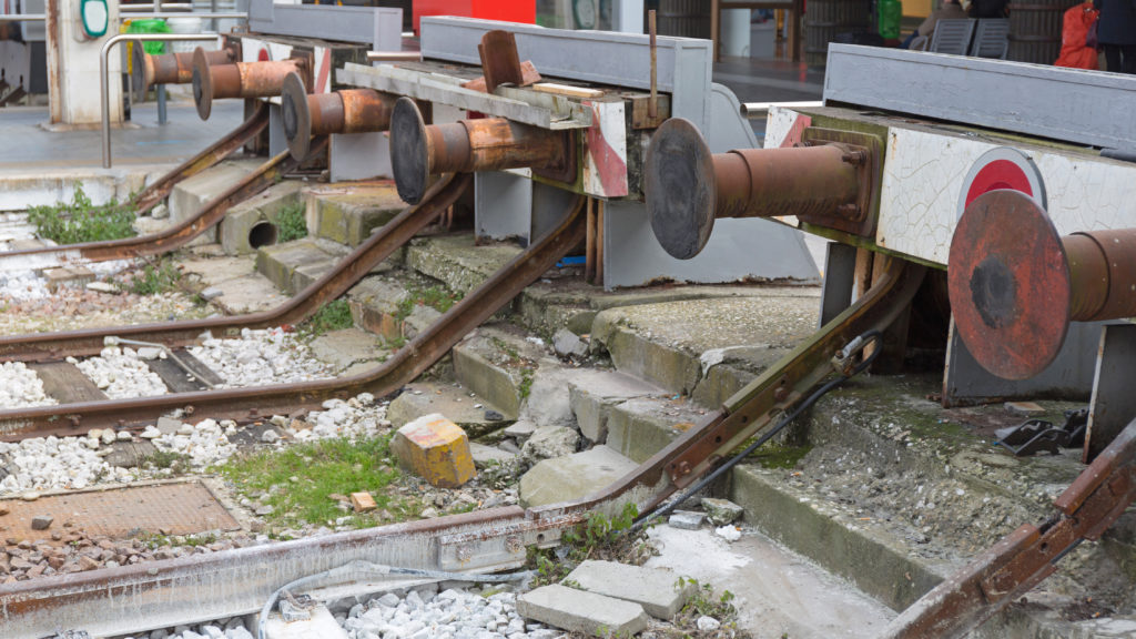 Train platform buffers absorb excess energy in a crash (Source: Shutterstock)
Because Kafka uses a store and forward design, it can act as a buffer between volatile external data sources and the Cassandra database, to prevent Cassandra from being overwhelmed by large data surges and ensure no data is lost. We plan to explore the Kafka as a buffer use case further, including how to optimize resources for Kafka and Cassandra for different sized loads (average, peaks, and durations); the impact on performance and business metrics of using Kafka as a buffer; and how to scale resources dynamically (autoscaling, elasticity). This blog covered other Kafka use cases, and this blog focused on the re-processing use case.
We plan to use “Anomalia Machina” for benchmarking Apache Kafka and Cassandra working together at massive scale and will try and get some “Big” numbers for throughput in particular to demonstrate solutions to some of the difficult issues that only arise at real scale. Using Kafka as a buffer will help with this goal as we’ll be able to resource Cassandra for a high average load, but then test the system out with increasingly higher and longer load spikes which will hopefully be absorbed by Kafka. This is likely to be more efficient and therefore cost-effective compared with statically increasing the Cassandra resources to cope with the load peak.
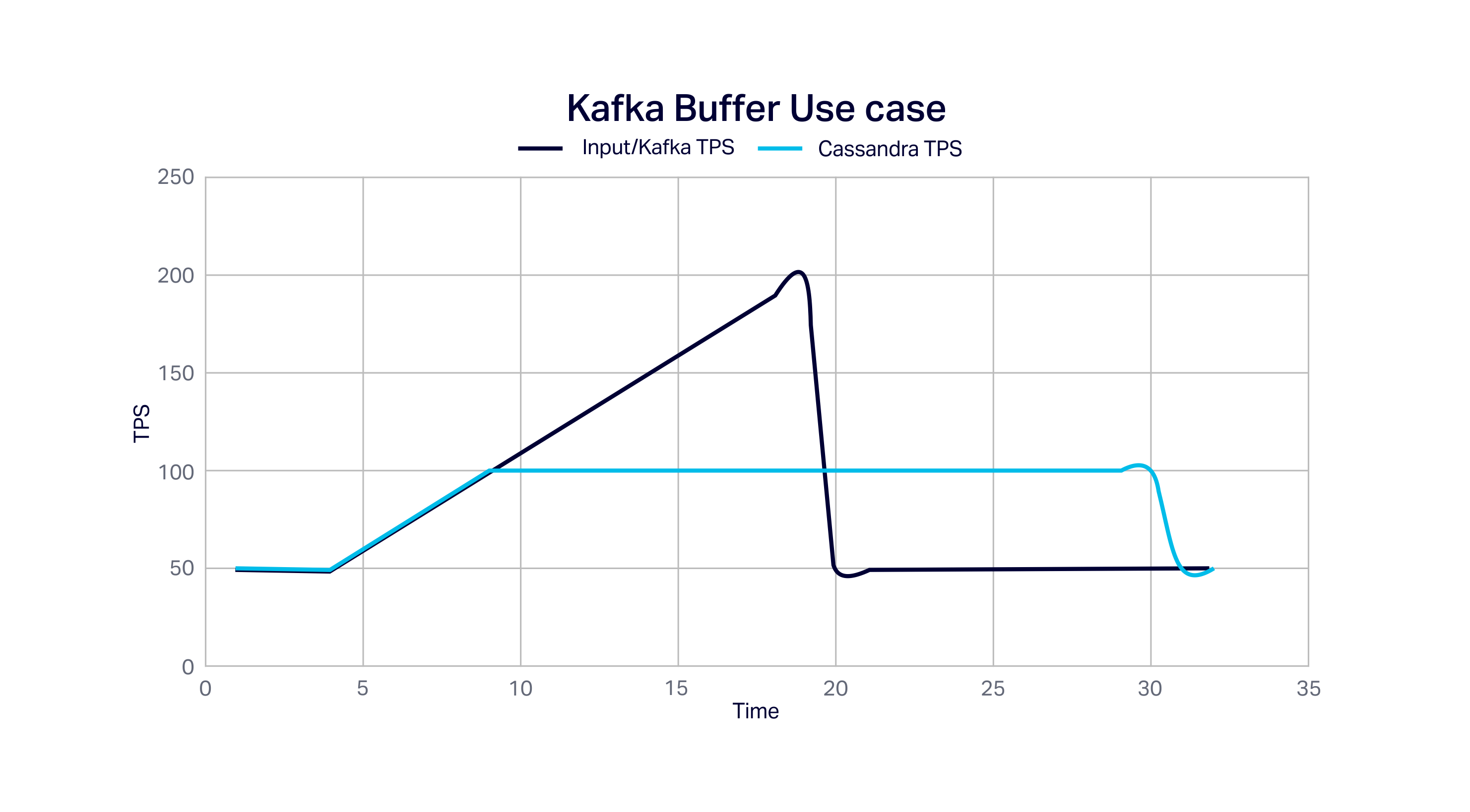
The following graph shows an example of Kafka as a Buffer Use Case in action. We assume Kafka has a maximum capacity double that of Cassandra (200 TPS c.f. 100 TPS), and that the input load ramps up from an average of 50TPS to 200TPS and then drops back to 50TPS at time 20. The events occurring above 100TPS are buffered by Kafka, enabling Cassandra to process the events at its maximum rate of 100TPS until it catches up again:
1.2 Scalability
We’ll be using Instaclustr’s managed Apache Kafka and Cassandra services (initially on AWS) for testing and benchmarking. In order to run the system at scale, we’ll also need to ensure that:
- The Kafka load generator is scalable and has sufficient resources to produce the high loads and patterns (e.g. load spikes of increasing duration)
- Performance and business metrics instrumentation, collection, and reporting is scalable
- That the application code used to write the data from Kafka to Cassandra, and the streams processing code including reading data from Cassandra, is scalable and has sufficient resources
- The Cassandra database is initially populated with sufficient data to ensure that reads are predominantly from disk rather than cache for added realism. This may take considerable time as a warm-up phase of the benchmark, or we may be able to do it once and save the data, and restore the data each time the benchmark is run or to populate new clusters.
We, therefore, plan to explore and trial technologies that are relevant for application scalability, for example, Open Source Microservices Frameworks.
1.3 Deployment Automation
There will be several moving parts for this project including the Apache Kafka and Cassandra clusters, Kafka load generator, application code, benchmarking harness, and metrics collection and analysis. It is possible to set up each of these manually (and creating Kafka and Cassandra clusters is easy with the Instaclustr console), however, we may have to do this multiple times for different clusters (sizes and combinations). There is also some effort required to configure interoperability settings each time a change is made.
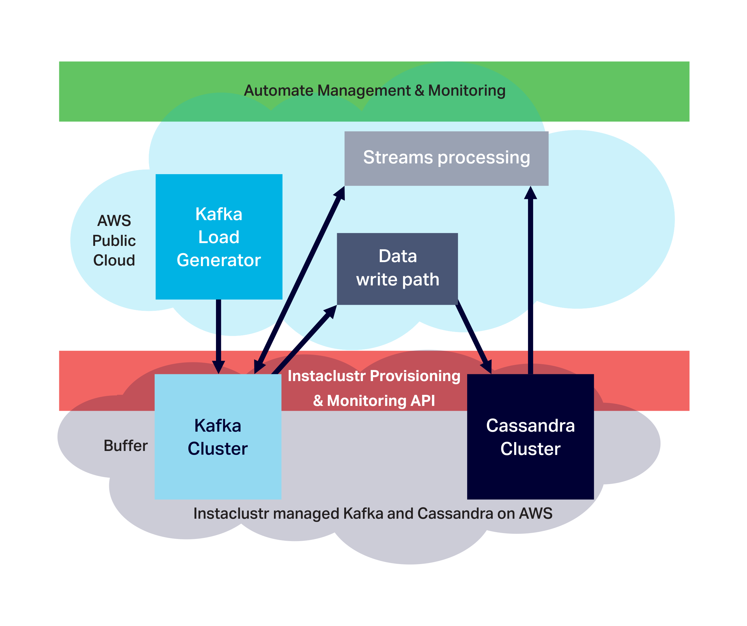
We, therefore, plan to investigate automation of provisioning, deployment, configuration, setup, running, and monitoring of the clusters, application, and benchmarking harness and metrics. Instaclustr has provisioning and monitoring APIs so we’ll start out by showing how these can be used to make the process more automatic and repeatable.
Here’s an overview of the main components, where they will be deployed, and the grand plan for automation:
2. Functionality
Let’s look at the application domain in more detail. In the previous blog series on Kongo, a Kafka focused IoT logistics application, we persisted business “violations” to Cassandra for future use using Kafka Connect. For example, we could have used the data in Cassandra to check and certify that a delivery was free of violations across its complete storage and transportation chain.
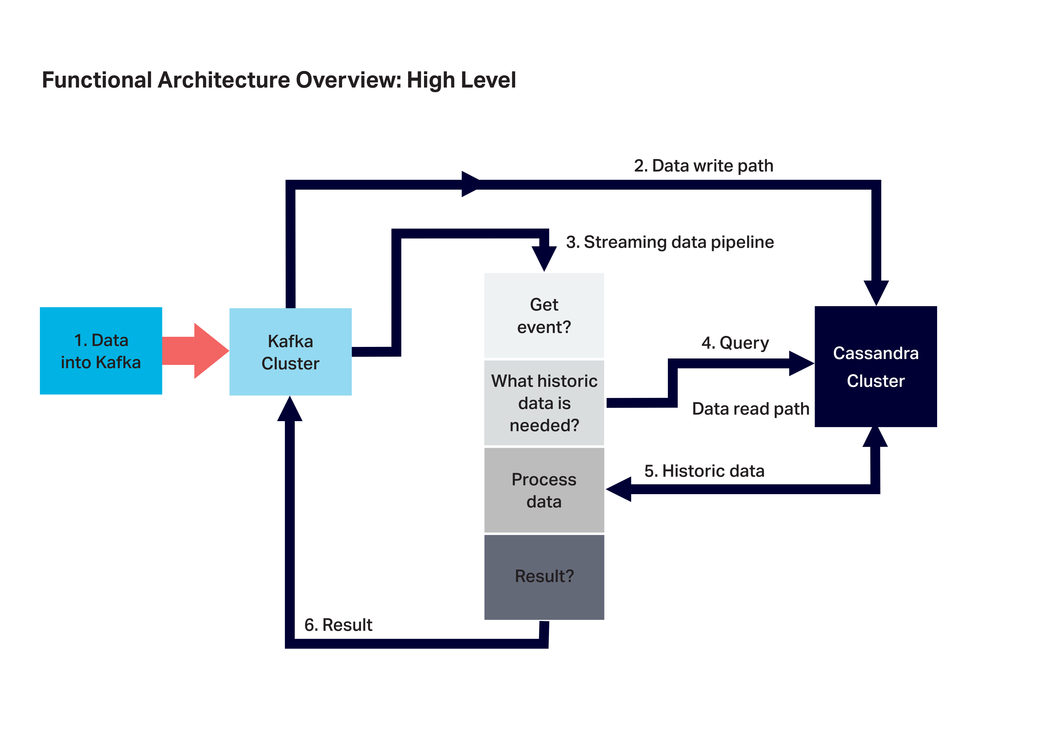
An appropriate scenario for a Platform application involving Kafka and Cassandra has the following characteristics:
- Large volumes of streaming data is ingested into Kafka (at variable rates)
- Data is sent to Cassandra for long term persistence
- Streams processing is triggered by the incoming events in real-time
- Historic data is requested from Cassandra
- Historic data is retrieved from Cassandra
- Historic data is processed, and
- A result is produced.
2.1 Anomaly Detection
 One of these things is not like the others… (Source: Shutterstock)
What sort of application combines streaming data with historical data with this sort of pipeline? Anomaly detection is an interesting use case. Anomaly detection is applicable to a wide range of application domains such as fraud detection, security, threat detection, website user analytics, sensors and IoT, system health monitoring, etc.
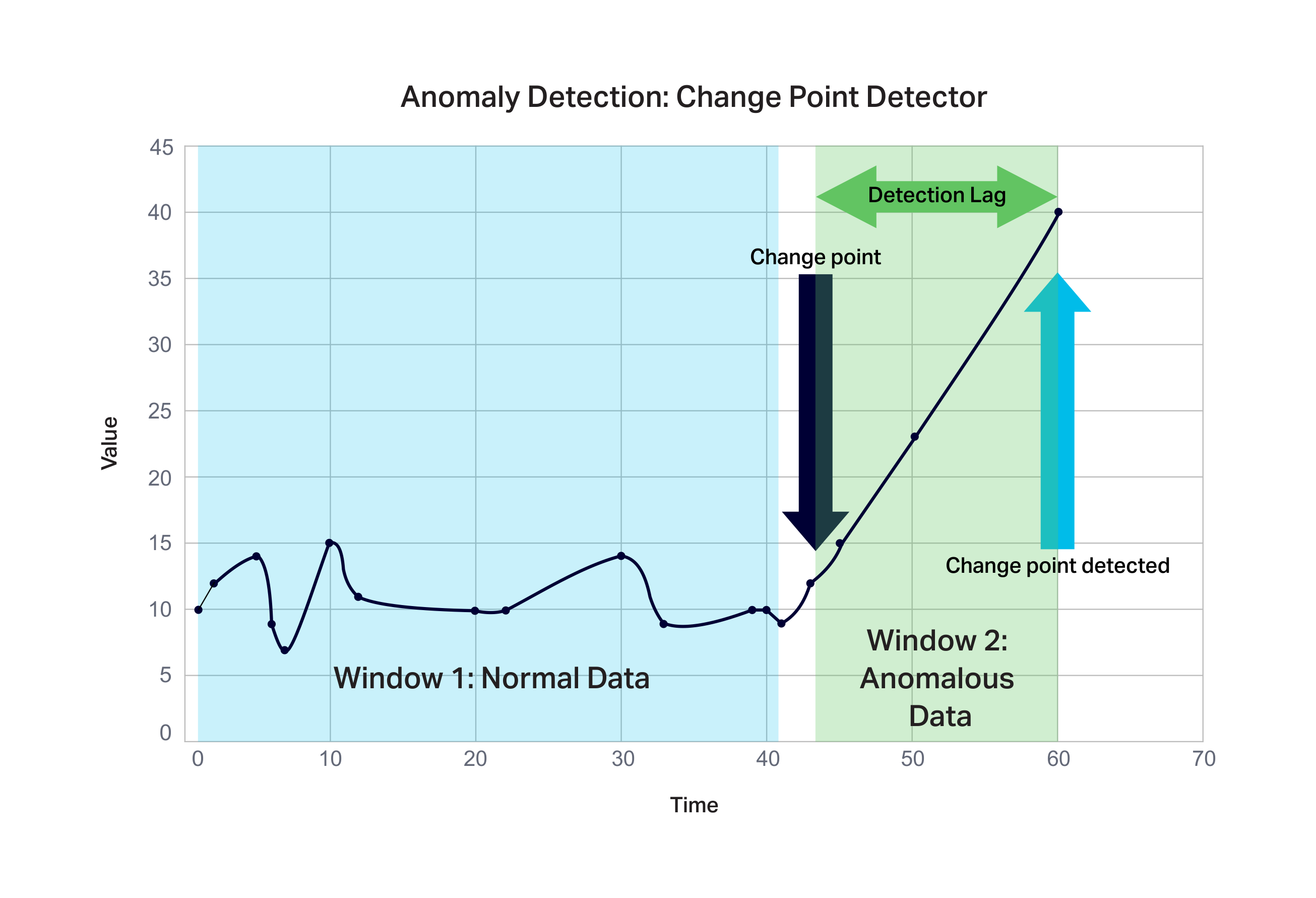
A very simple type of unsupervised anomaly detection is Break or Changepoint analysis. This takes a stream of events and analyses them to see if the most recent transaction(s) are “different” to previous ones, and works like this:
- The simplest version is a single variable method, which just needs data from the variable of interest (e.g. an account number, an IP address, etc.), not other variables.
- The data doesn’t need to be equally temporally spaced, so it may extend over a long period of time and, making the query more demanding (i.e. the earlier data is more likely to be on disk rather than in cache).
- The amount of events needed may be dynamic and depend on the actual values and patterns, and how accurate the prediction needs to be.
- The prediction quality is measured by accuracy, a confusion matrix, and how long it takes to detect a change point after it first occurred. In reality, the algorithms typically work by dividing the data into 2 windows—1 window is “normal” data before the change point, the second is “abnormal” data after a change point. The amount of data in the second window is variable resulting in the detection lag.
The following diagram shows an example of the detection of a change point at time 60, 3 data points after the identified change point:
We’ll start with the simplest possible anomaly detection approach, and possibly extend it later (e.g. to multivariate, or categorical rather than just numerical values). CUSUM is a good start. It dates from the 1950’s from cybernetic industrial control systems (cybernetics morphed into neural networks which made a surprise come back and became the dominant machine learning technology for big data), and it’s still applicable to some problems. We’ll treat it as a black box which takes a new event, queries historic data, and outputs anomaly detected/not detected. We used this blog as a starting point for the CUSUM code, but modified it to build a new model each time using historic data, and allow changes to be detected in both positive and negative directions.
Different approaches to anomaly detection are supervised/unsupervised, this is an unsupervised approach (i.e. no training data and no model) which uses the raw historic data. This will be more demanding in terms of the frequency and amount of data read from Cassandra. We can also tune the read:write operations ratio for the system by varying the probability of each new event triggering the anomaly detector pipeline, perhaps based on some pre-processing to decide if the event is high risk or not (e.g. based on frequency or value).
We’ll start with a very simple CUSUM which processes numeric <key, value> data pairs. The key is a numeric ID (e.g. representing say a bank account, or the client IP address of a web interaction), and the value is numeric representing the amount of the transaction or the number of web pages visited in a visit etc). There are algorithms that work for categorical (e.g. String) data which we may investigate in the future to enrich the use case (e.g. extra data available may be geographical locations or URLs etc.).
2.2 Data models
Given the simple <key, value> data records, what will the data models look like for Kafka and C*?
For Kafka, we’ll use a single topic with <key, value> records. Using a key means we’ll need multiple partitions for the topic so we can have multiple consumers reading the data for scalability.
The <key, value> pairs will be persisted to Cassandra. Using a naive schema with a primary key consisting of a single partition key as the record key will result in a problem. Only a single value will be retained for each unique key (as new values will replace the old value), a query will only ever return a single value, and lots of “tombstones” will be created! The obvious solution is to treat the data as a time series and add the Kafka record timestamp (created by the Kafka producer) as a clustering key in the primary key as follows (id is the partition key, time is the clustering key):
create table data_stream (
id bigint,
time timestamp,
value double,
Primary key (id, time, value)
) with clustering order by (time desc);
This allows us to store multiple values for each key, a value for each unique combination of <key, timestamp> (assuming the timestamp is different for each value), and then allows us to retrieve up to a specified maximum number of records in reverse order for a specific key using a where clause, e.g.
SELECT * from data_stream where id=1 limit 10;
 id | time                            | value

----+---------------------------------+-------

  1 | 2018-08-31 07:12:53.903000+0000 | 75966

  1 | 2018-08-31 07:12:02.977000+0000 | 94864

  1 | 2018-08-30 02:12:02.157000+0000 | 93707

  1 | 2018-08-30 01:11:36.219000+0000 | 42982

  1 | 2018-08-29 08:11:13.209000+0000 | 42011

  1 | 2018-08-28 05:10:46.198000+0000 | 42037

  1 | 2018-08-27 05:10:02.562000+0000 | 12662

  1 | 2018-08-26 04:09:38.671000+0000 |   443

  1 | 2018-08-20 01:03:53.151000+0000 | 95385

  1 | 2018-08-10 05:03:38.129000+0000 | 78977
To insert the records in Cassandra we simply do an insert (with appropriate record key, timestamp, and value supplied from Kafka):
INSERT into data_stream (id, time, value) values (?, ?, ?)
Note that this schema results in unbounded partitions, so in real life, we’d also have a TTL or use buckets to limit partition sizes (Watch out for Cassandra’s Year 2038 TTL problem and a fix).
3. Cassandra Test Implementation
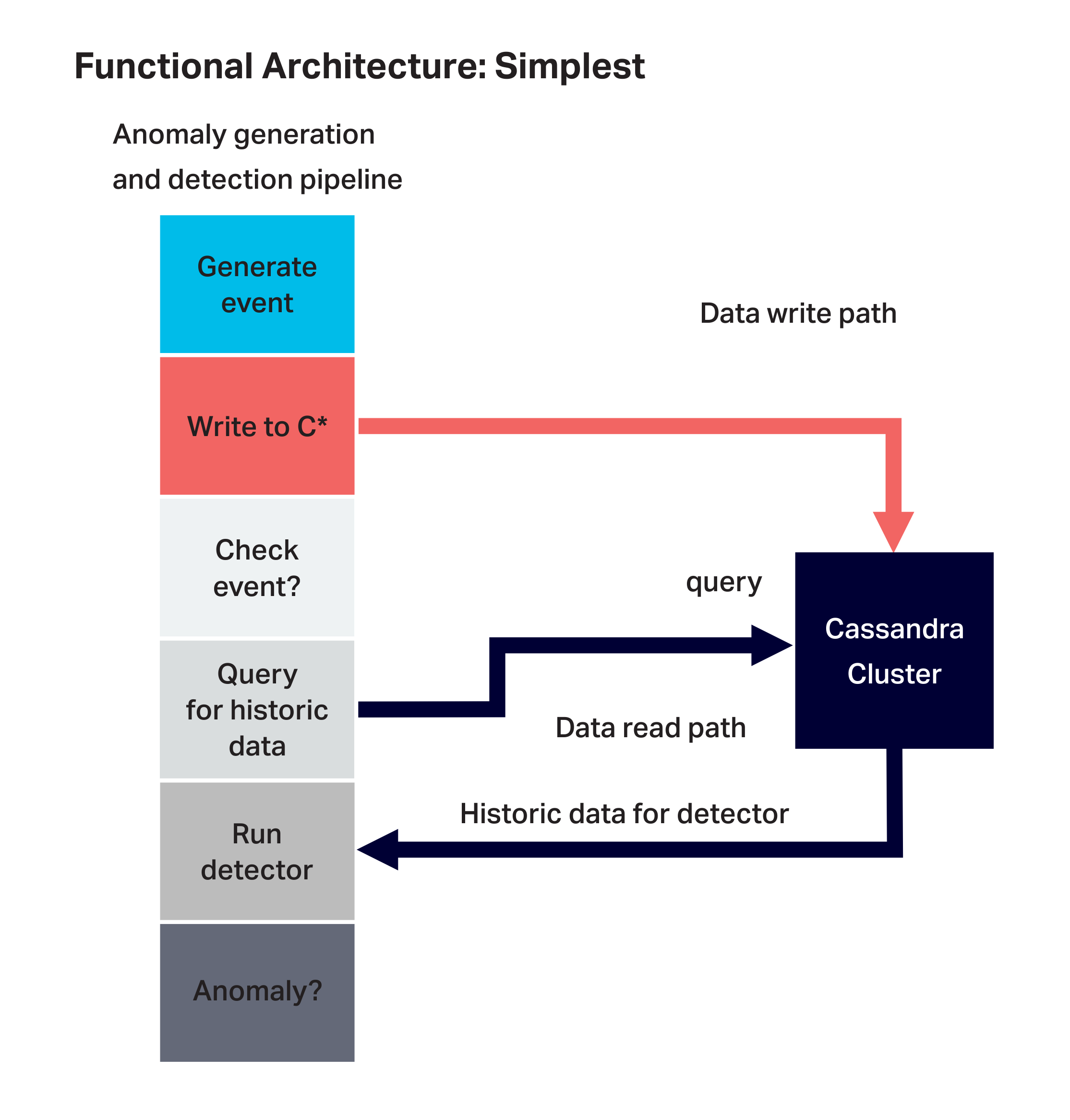
We started building the application incrementally and wrote an initial test application using Cassandra only. We wrote an event generator based on a random walk which produces “interesting” data for the anomaly detector to look at, it can be tuned to produce more or less anomalies as required. This event generator was included in a simple Cassandra client and used to trigger the anomaly detection pipeline and write and read paths to Cassandra:
3.1 Initial Cassandra Results
In order to check that the anomaly pipeline is working correctly and to get an initial idea of the resource requirements for the pipeline application and baseline performance of the Cassandra cluster, we provisioned a small Cassandra cluster on Instaclustr on AWS using the smallest recommended Cassandra production AWS instances and a large single client instance as follows:
- Cassandra Cluster: 3 nodes x 2 cores per node, EBS tiny m4l-250:
- 8GB RAM, 2 cores, 250GB SSD, 450 Mbps dedicated EBS b/w.
- Client Instance: c5.2xlarge:
- 8 cores, 16GB RAM, EBS b/w up to 3,500 Mbps.
We also wanted to explore the relationship of a few parameters and metrics including event generation rate, write rate, anomaly check rate, read:write ratio, and data write/read rate. By increasing the number of Cassandra client application threads we can increase the event generation rate up to the maximum sustainable rate for the Cassandra cluster. Every event generated is written to Cassandra, giving the write rate (1:1 ratio with generation rate).
For each generated event there is a probability of running the anomaly detection pipeline.
- 1:1 read:write operations ratio: If the probability is 1.0 then a read to Cassandra is issued for the most recent 50 rows for the event key. The read:write operations ratio is 1:1, but 50 times more rows are read than written.
- 0:1 read:write operations ratio: If the probability is 0 then no checking is ever performed so there are no reads and the load is write only, giving a read:write ratio of 0:1.
We’ll run load tests for these 1:1 and 0:1 options, and a 3rd where the probability of checking is 0.02 (1 in 50) which results in the same number of rows written and read, but a 1:50 read:write operation ratio (i.e. 1 read for every 50 writes).
The total throughput is the sum of write and read operations. The checking rate is the event generation rate times the probability of checking.
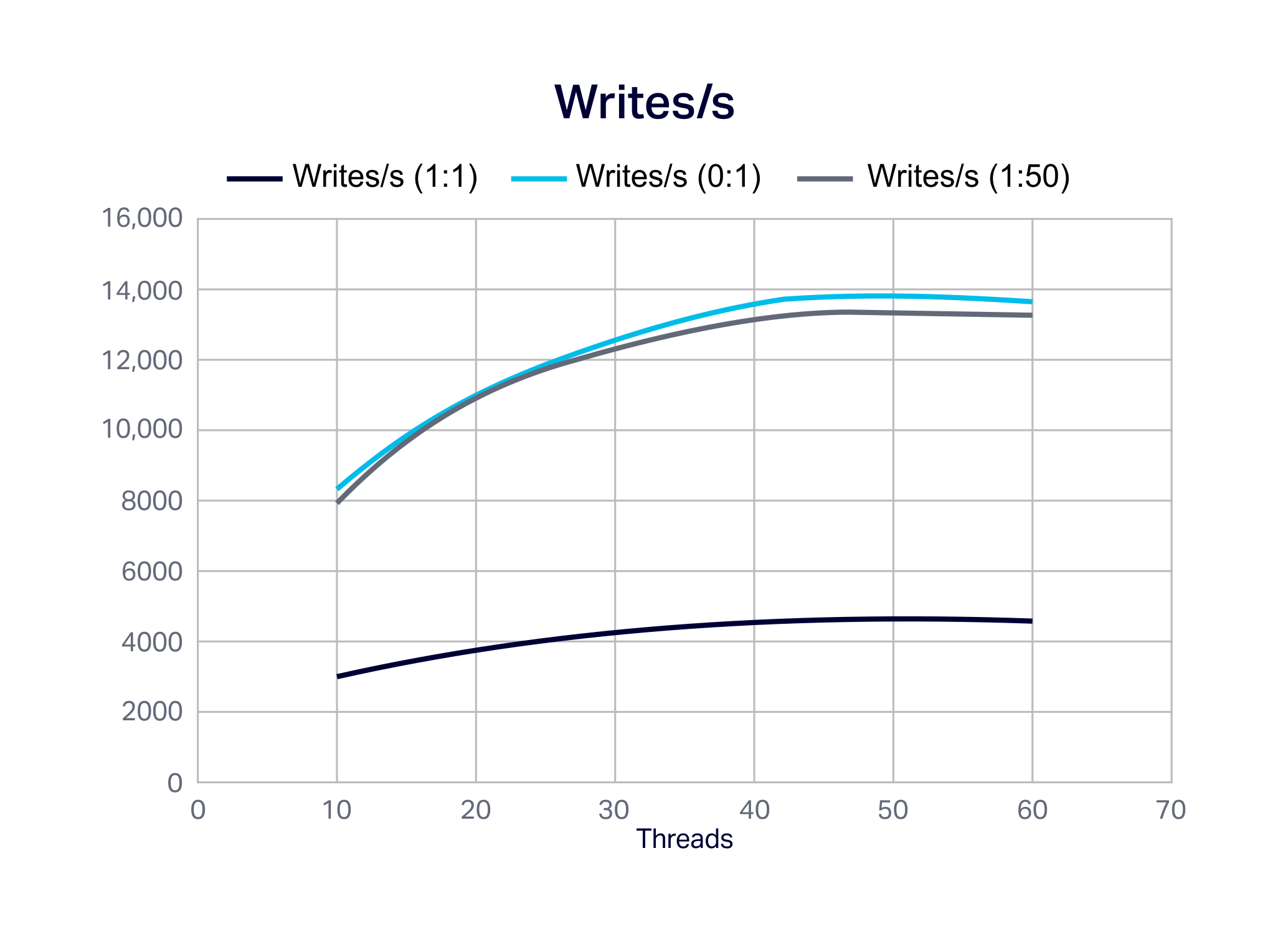
The following graph shows the increase in writes/s (identical to event generator rate) with increasing thread count. The maximum write rate is close to 14,000/s, achieved by the 0:1 scenario (Cassandra is better at writes than reads). The 1:50 case is slightly less and the 1:1 scenario only reaches 33% (4,600/s) of the maximum. The Cassandra cluster CPU utilization is at 100% by 45 threads, and the application client-server CPU is <= 20%.
 The next graph summarises operation/s for the maximum capacity for writes/s, reads/s, total/s and check/s for the 1:1 and 1:50 scenarios:
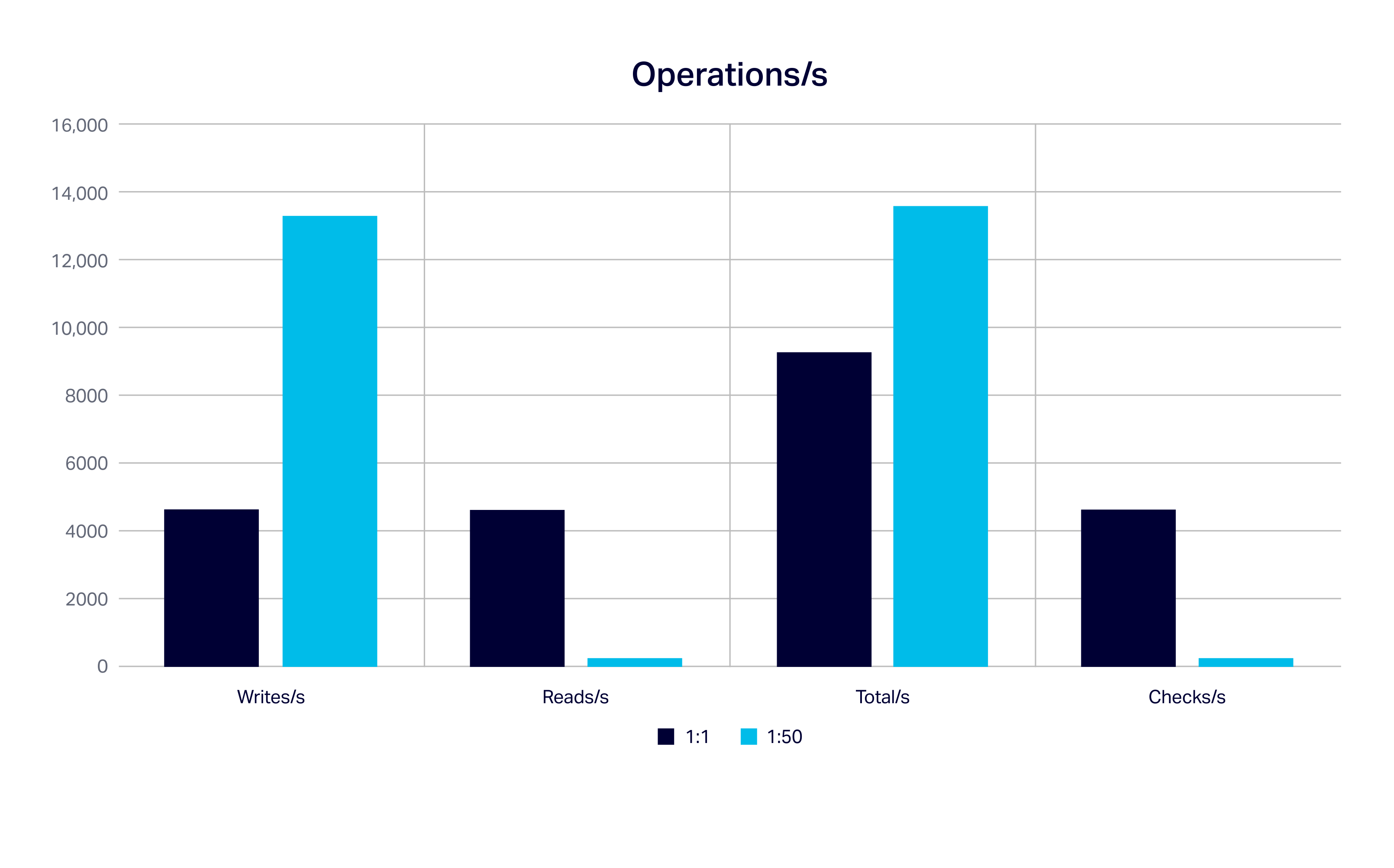 The 1:50 scenario has the best writes/s and total operation/s (close to 14,000), but the 1:1 scenario maximises read/s and checks/s (4,6000/s).
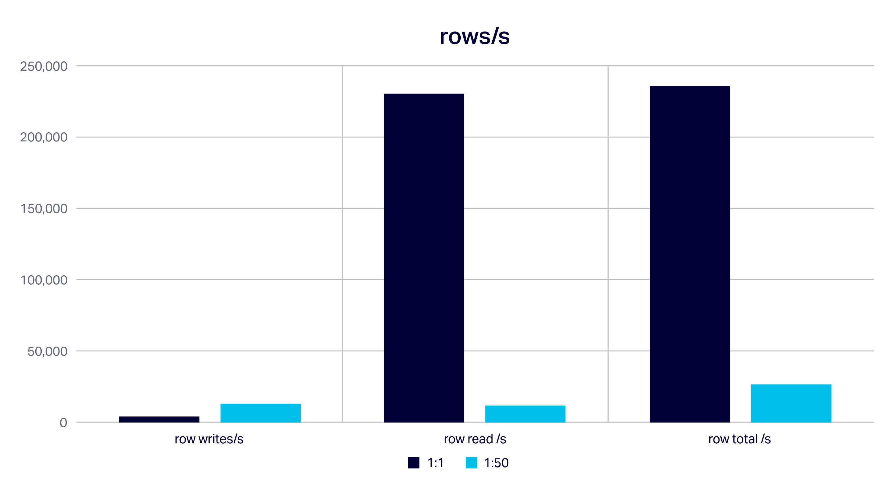
The next graph shows the rate for rows written, read and total for two scenarios. This shows that the 1:1 scenario is the most demanding and maximizes the total rows (235k/s) and rows read (230k/s) from Cassandra, as it reads substantially more rows than the 1:50 option. The 1:50 scenario only maximizes the number of rows written to Cassandra (13k/s).
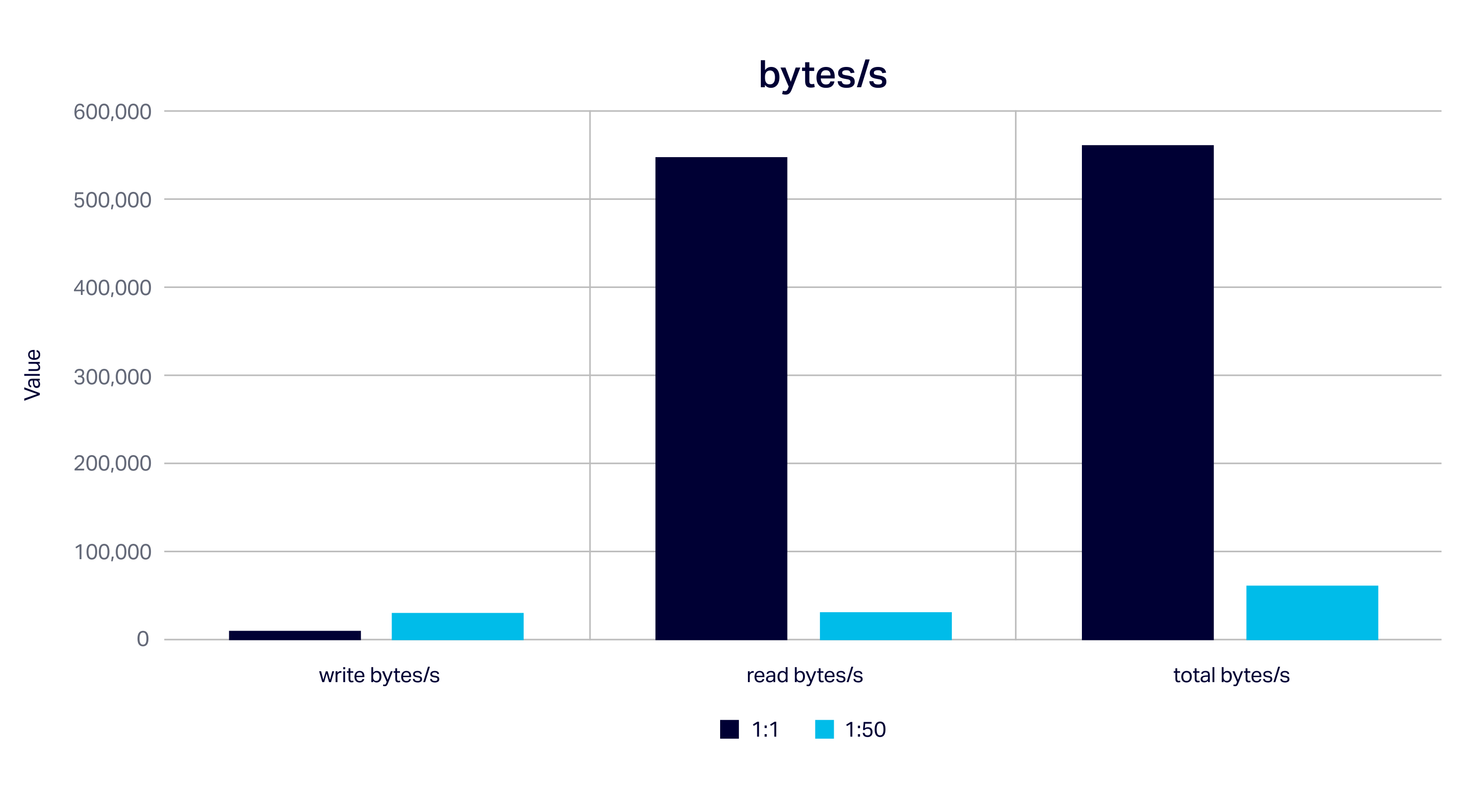
We get the same ratios looking at bytes/s written/read/total, but bigger numbers. The 1:1 scenario maximizes reads and total data in and out of Cassandra (5.6MB/s). The 1:50 scenario writes the most data to Cassandra (0.3MB/s).
Here’s a summary of the maximum values for the scenarios and metrics:
| Scenario/Metric | Maximum |
| 1:50 writes/s | 13,274 |
| 1:50 total/s | 13,545 |
| 1:1 checks/s | 4,615 |
| 1:1 total rows/s | 235,365 |
| 1:1 row reads/s | 230,750 |
| 1:50 row writes/s | 13,274 |
| 1:1 total MB/s | 5.6 |
| 1:1 read MB/s | 5.5 |
| 1:50 write MB/s | 0.318 |
We’ll use these values as a (probably optimistic, given the simplified anomaly detection pipeline, and that we didn’t have much data in Cassandra) baseline for comparing the next version of Anomalia Machina against (to check that we’re getting close to the maximum throughputs expected), deciding what parameter settings to use and metrics to report for benchmarking, and for selecting appropriate larger instances sizes and numbers of nodes for the bigger benchmarking.
Over the next few blogs we’ll explain how the combined Kafka+Cassandra version of Anomalia Machina works, reveal the initial results, and explore our initial attempts at automation.
4. Further Resources
- Anomaly Detection https://en.wikipedia.org/wiki/Anomaly_detection
- Change Detection https://en.wikipedia.org/wiki/Change_detection
- An introduction to Anomaly Detection, https://www.datascience.com/blog/python-anomaly-detection
- A Survey of Methods for Time Series Change Point Detection 10.1007/s10115-016-0987-z
- A review of change point detection methods https://arxiv.org/pdf/1801.00718.pdf
- Unsupervised real-time anomaly detection for streaming data https://doi.org/10.1016/j.neucom.2017.04.070
- Anomaly Detection With Kafka Streams https://dzone.com/articles/highly-scalable-resilient-real-time-monitoring-cep
- Building a Streaming Data Hub with Elasticsearch, Kafka and Cassandra (An Example With Anomaly Detection) https://thenewstack.io/building-streaming-data-hub-elasticsearch-kafka-cassandra/
- Real-time Clickstream Anomaly Detection with Amazon Kinesis Analytics https://aws.amazon.com/blogs/big-data/real-time-clickstream-anomaly-detection-with-amazon-kinesis-analytics/