In Part 2 of this series, we introduced the steps needed for batch training in TensorFlow with some example Python code. In this next part we’ll have a look at some performance metrics and explore the results.
1. Performance Metrics

Sometimes accuracy is all that matters! (Source: Shutterstock)
It took me a reasonable amount of time to get to this point, due to a combination of factors, but mainly because it was hard to understand how well the models were performing. After I included the following metrics, things began to make more sense.
Here’s the list of metrics that can be included in training and evaluation results, and here some of the more useful metrics. some of the more useful metrics.
Accuracy—also called “Classification Accuracy”—is a value from 0 (useless) to 1.0 (perfect) and it’s computed as the ratio of the number of correct predictions to the total number of samples. However, it can be misleading and only works well if there are an approximately equal number of samples in each class; you want accuracy to increase with training.

Biodiversity loss includes species extinction—the Tasmanian Tiger (Thylacine) became extinct in 1936 (Source: https://commons.wikimedia.org/wiki/File:Thylacine.png)
Loss in TensorFlow is not a metric since you want the loss to decrease with training. Loss functions are not technically metrics either as they are more focused on the internal performance of the model itself, and often relate to the type of model used. For neural network models (which TensorFlow supports) the training and model optimization process is designed to minimize a loss function.
You may notice that the TensorFlow metric links are actually for a thing called “Keras.”
What’s this? Well, Keras is a simpler deep learning library, using Python, which runs on top of TensorFlow. If you need more control, then there are low-level APIs in TensorFlow. (TensorFlow itself is written in a combination of Python, C++, and CUDA—CUDA is a GPU programming language to enable general-purpose computing on GPUs.)
Ok, back to metrics.
A Confusion Matrix can reduce confusion—confused? (Source: Shutterstock)
Confusion Matrix
A confusion matrix is a common way of summarizing model accuracy for binary classification problems (the class being learned is simply TRUE or FALSE). It’s a simple 2×2 matrix containing counts. The rows are the actual classes (TRUE/FALSE), and the columns are the predicted classes. The values in the cells are the counts that satisfy both.
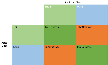
It’s not directly available in TensorFlow, but the individual metrics are available for each cell as follows:
TruePositives—top left cell, the number of samples that are TRUE and correctly predicted TRUE
TrueNegatives—bottom right cell, the number of samples which are FALSE and correctly predicted FALSE
FalseNegatives—top right cell, the number of samples which are TRUE but incorrectly predicted FALSE
FalsePositives—bottom left cell, the number of samples which are FALSE but incorrectly predicted TRUE
These metrics are particularly useful for learning in problem domains where there may be a disproportionate cost for missing/ignoring some positives (FalseNegatives), e.g., fraud detection, or misdiagnosing some negatives (FalsePositives), e.g., in medicine where a cure may have harmful side-effects and should not be used unless a diagnosis is certain.
Accuracy can also be computed as

Some previous blogs that explained accuracy and confusion (and more, including precision and recall etc.) in the context of Spark ML are here and here.
2. Example Trace
So now let’s have a look at a trace of an example run on 1 week of drone delivery data, which had the same simple shop busy/not busy rule applied for the entire week (i.e., there was no concept drift in the week of data).
|
1 2 3 4 5 6 7 8 9 10 11 12 13 14 15 16 17 18 19 20 21 22 23 24 25 26 27 28 29 30 31 32 33 34 35 36 37 38 39 40 41 42 43 44 45 46 47 48 49 50 51 52 53 54 55 56 57 58 59 60 61 62 63 64 65 66 67 68 69 70 71 72 73 74 75 76 77 78 79 80 81 82 83 |
python3 dronebatch.py class shop_id shop_type shop_location weekday hour avgTime avgDistance avgRating another1 another2 another3 another4 another5 0 0 1 19 10 1 1 44 5 1 2 99 3 17 852 1 1 2 7 8 1 1 27 19 3 2 45 8 18 801 2 0 3 17 15 1 1 47 20 4 1 97 12 10 285 3 1 4 1 12 1 1 24 9 5 2 55 2 11 225 4 1 5 14 10 1 1 48 1 2 1 10 10 15 843 dtype: object records 5600 columns 14 class 0 2660 class 1 2940 Number of training samples: 3360 Number of testing samples: 2240 _________________________________________________________________ Layer (type) Output Shape Param # ================================================================= dense (Dense) (None, 128) 1792 dropout (Dropout) (None, 128) 0 dense_1 (Dense) (None, 256) 33024 dropout_1 (Dropout) (None, 256) 0 dense_2 (Dense) (None, 128) 32896 dropout_2 (Dropout) (None, 128) 0 dense_3 (Dense) (None, 1) 129 ================================================================= Total params: 67,841 Trainable params: 67,841 Non-trainable params: 0 _________________________________________________________________ None Epoch 1/200 105/105 [==============================] - 1s 2ms/step - loss: 6.5520 - accuracy: 0.5077 - true_positives: 995.0000 - true_negatives: 711.0000 - false_positives: 849.0000 - false_negatives: 805.0000 … Epoch 125/200 105/105 [==============================] - 0s 1ms/step - loss: 0.2763 - accuracy: 0.8813 - true_positives: 1615.0000 - true_negatives: 1346.0000 - false_positives: 214.0000 - false_negatives: 185.0000 testing... 70/70 [==============================] - 0s 960us/step - loss: 0.2864 - accuracy: 0.8862 - true_positives: 1064.0000 - true_negatives: 921.0000 - false_positives: 179.0000 - false_negatives: 76.0000 [0.28635311126708984, 0.8861607313156128, 1064.0, 921.0, 179.0, 76.0] |
What’s going on here? For a start, there are roughly equal numbers of busy/not busy observations. This turned out to be critical, as if the numbers are too unbalanced then the accuracy metric is telling you nothing useful—i.e., if there’s a 95% chance of a not busy observation then you can just guess and get approximately 0.95 accuracy. I had this problem early on so ended up having to change the rules to get an approximately 50/50 balance. There are workarounds if you are stuck with an unbalanced class distribution.
Next, the accuracy of the model improved from 0.5 to 0.88 after 125 training epochs, a significant improvement, and we didn’t need to use the whole 200 epochs. The confusion metrics tell us that this accuracy is actually pretty good, there are far more true positives and negatives than false ones.
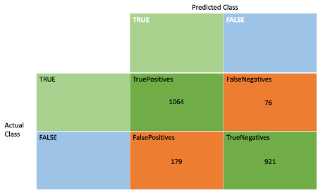
Finally, the evaluation against a different subset of data provides reassurance that the model hasn’t been overfitted. The accuracy is 0.88, and again the true positives and negatives outweigh the false ones. Here’s the evaluation confusion matrix:
3. Measuring Training Time and Changing Batch Size

(Source: Shutterstock)
It didn’t seem very “scientific” just showing the results of a single ML trace (and in reality, I had many runs to get to this point). I was also interested in knowing how long training takes (even with such as small data sample), how repeatable the training is even with the same settings, and if batch size makes much difference to training time or accuracy etc.
So, I added the following code to accurately measure the process specific time for the fit() function:
|
1 2 3 4 5 |
start_t_ns = time.process_time_ns() model.fit(drone_features, drone_labels, batch_size=BATCH_SIZE, epochs=EPOCHS, callbacks=[callback]) end_t_ns = time.process_time_ns() time_diff = end_t_ns - start_t_ns print("training time (ns) = ", time_diff) |
This is the most accurate approach to time measurement in Python according to this blog.
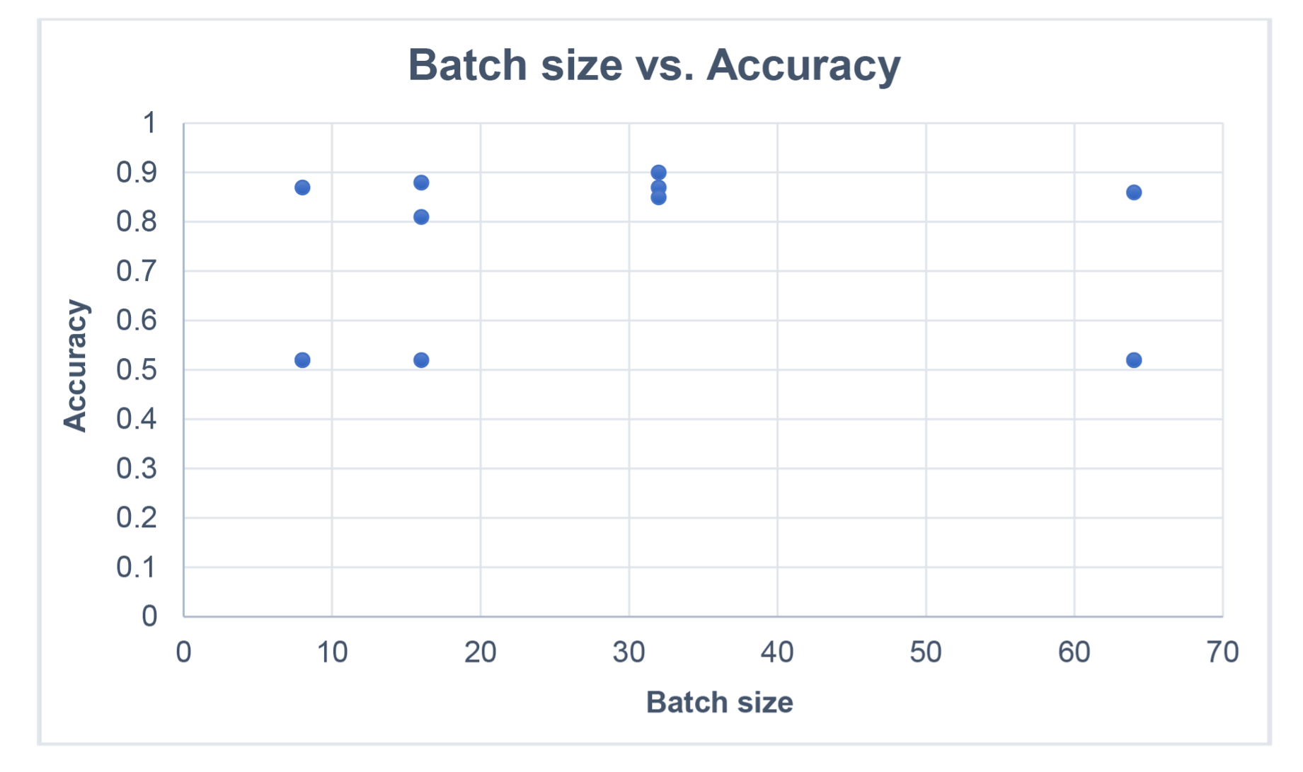
Next, I did 3 training runs with increasing batch size (from 8 to 64) and plotted the results. The 1st graph is for accuracy. The most obvious observation is that in some training runs the accuracy is not very good, and overall, there’s a wide spread from 0.5 to 0.9. The results for a batch size of 32 are more consistent, around 0.85 to 0.9. (but this could be luck!).
The 2nd graph shows the training time in seconds. Again, there’s a wide spread from 5 to 92 seconds.
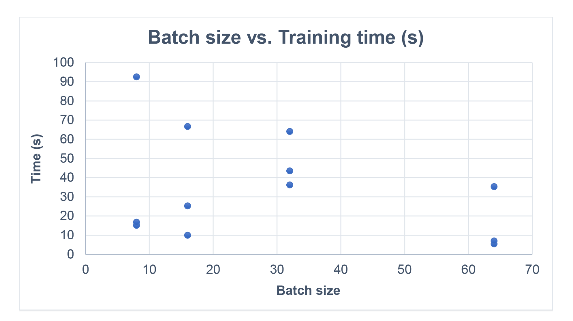
What’s actually going on here? Basically, for some runs, the training stops very quickly as the optimization gets stuck in a bad local minima—corresponding to results with low accuracy. Ideally you want to find the global minimum which corresponds to the optimal solution, but optimization may find a local minima which isn’t optimal and is difficult to move away from—there’s a nice 3D diagram showing this here. This is a bit like trying to find your way to the centre of a maze but getting stuck in dead ends and having to backtrack!
Try not to get stuck in a dead-end local minima (Source: Shutterstock)
Here’s a good blog that explains more about the effect of batch size on training dynamics. Another obvious conclusion to draw from all of these results is that each training run is not repeatable. This is because we are doing random sampling (shuffling) of the training set from the available data, which likely contributes to the variation in results for the larger batch sizes (from the above blog):
“Large batch size means the model makes very large gradient updates and very small gradient updates. The size of the update depends heavily on which particular samples are drawn from the dataset. On the other hand, using small batch size means the model makes updates that are all about the same size. The size of the update only weakly depends on which particular samples are drawn from the dataset.”
So, this seems like a good start to our ML experiments. What have we learned so far? Even though this isn’t a lot of training data (I had to simplify my rules several times to ensure sufficient accuracy with around 6000 observations), a large number of auto epochs, smaller batch size, and balanced class distributions can result in good results—up to 90% accuracy. But remember to look at the confusion metrics for a sanity check, and maybe do multiple training runs (saving the parameters and selecting/loading the best result) if you are sampling the training data randomly. It can take up to a minute to train a model even with this small quantity of data, so we’ll need to take training time into account as move onto potentially more demanding real-time training scenarios.
In Part 4 of this series, we’ll start to find out how to introduce and cope with concept drift in the data streams, try incremental TensorFlow training, and explore how to use Kafka for Machine Learning.
Follow the series: Machine Learning Over Streaming Kafka® Data
Part 2: Introduction to Batch Training and TensorFlow
Part 3: Introduction to Batch Training and TensorFlow Results
Part 4: Introduction to Incremental Training With TensorFlow
Part 5: Incremental TensorFlow Training With Kafka Data
Part 6: Incremental TensorFlow Training With Kafka Data and Concept Drift