One of the goals of incremental learning is to train a model continuously from streaming data. Incremental learning from streaming data means you don’t need all the data in memory at once, and the model is as up-to-date as possible, which can matter for real-time use cases. The third driver for incremental learning that I mentioned in the previous blog is when there is concept drift in the data itself—but we’ll ignore this aspect for the time being.

Incremental clicker games can be addictive. The kinds involving performing simple actions repeatedly to gain higher levels. (Source: Shutterstock)
In the last blog we demonstrated batch training with TensorFlow, and mentioned that TensorFlow, being a neural network framework, has the potential for incremental learning—just like animals and people do. In this blog, we will set ourselves the task of using TensorFlow to demonstrate incremental learning from the same static drone delivery data set of busy/not busy shops that we used in the last blog.
Let’s take a look of the modified Python TensorFlow code.
1. Incremental TensorFlow Example
Everything starts out the same as before:
|
1 2 3 4 5 6 7 8 9 10 11 12 13 14 15 16 17 18 19 20 21 22 23 24 25 26 27 28 29 30 31 32 33 34 35 36 37 38 39 40 41 42 43 44 45 46 47 48 49 50 51 52 53 54 55 56 57 58 59 60 61 62 63 64 65 66 67 68 69 70 71 72 73 74 75 76 77 78 79 80 81 82 83 84 85 86 87 88 89 |
import os from datetime import datetime import time import threading import json from sklearn.model_selection import train_test_split import pandas as pd import numpy as np import tensorflow as tf import tensorflow_io as tfio # incremental learning experiment # idea is to use a small number of records at a time to train the model incrementally DCOLUMNS = [ # labels 'class', 'shop_id', 'shop_type', 'shop_location', 'weekday', 'hour', 'avgTime', 'avgDistance', 'avgRating', 'another1', 'another2', 'another3', 'another4', 'another5' ] print('Incremental learning on 1 week of drone data') fname = 'week1.csv' drone_iterator = pd.read_csv(fname, header=None, names=DCOLUMNS, chunksize=100000) drone_df = next(drone_iterator) print(drone_df.head()) print("size ", drone_df.size) print("data types ", drone_df.dtypes) l1 = len(drone_df) l2 = len(drone_df.columns) l3 = len(drone_df[drone_df["class"]==0]) l4 = len(drone_df[drone_df["class"]==1]) print("records ", l1, " columns ", l2, " class 0 ", l3, " class 1 ", l4) |
The first difference is a decision on how much of the incoming data to use for training vs. testing. In this case, I’m going to use close to all the data available for training—with the potential risk of overfitting.
|
1 2 3 4 5 6 7 8 9 10 11 12 13 14 15 16 17 18 19 20 21 22 23 24 25 26 27 28 29 30 31 32 33 34 35 36 37 38 39 40 41 42 43 44 45 46 47 48 49 50 51 52 53 54 55 56 57 58 59 60 61 62 63 64 65 66 67 68 69 70 71 72 73 74 75 |
# use all the data for incremental training train_df, test_df = train_test_split(drone_df, test_size=0.00001, shuffle=False) print("Number of training samples: ", len(train_df)) print(train_df.head()) NUM_COLUMNS = len(train_df.columns) And as before, let’s build a model: # build model # Set the parameters OPTIMIZER="adam" LOSS=tf.keras.losses.BinaryCrossentropy(from_logits=False) METRICS=['accuracy', tf.keras.metrics.TruePositives(), tf.keras.metrics.TrueNegatives(), tf.keras.metrics.FalsePositives(), tf.keras.metrics.FalseNegatives()] # # 32 is the default BATCH_SIZE=32 EPOCHS=20 # design/build the model model = tf.keras.Sequential([ tf.keras.layers.Input(shape=(NUM_COLUMNS,)), tf.keras.layers.Dense(128, activation='relu'), tf.keras.layers.Dropout(0.2), tf.keras.layers.Dense(256, activation='relu'), tf.keras.layers.Dropout(0.4), tf.keras.layers.Dense(128, activation='relu'), tf.keras.layers.Dropout(0.4), tf.keras.layers.Dense(1, activation='sigmoid') ]) print(model.summary()) # compile the model model.compile(optimizer=OPTIMIZER, loss=LOSS, metrics=METRICS) |
This time we use all the data for training:
|
1 2 3 4 5 6 7 |
# use all data for training drone_features = drone_df.copy() drone_labels = drone_features.pop('class') |
So far this looks pretty similar to the batch learning code, but how do we simulate incremental learning? Well, the fundamental ideas behind incremental learning are using the most recent data for training, and repeating when more data becomes available. The other real-world constraint is that you don’t have to access to future data, so you can’t use it for training or evaluation. For my initial experiment I’m therefore going to extract a subset of observations from the available training data, in strict time order. We’ll use a fixed size to repeatedly train the model—remembering that the way fit() works is to update the model, rather than relearn from scratch. Here’s my training loop:
|
1 2 3 4 5 6 7 8 9 10 11 12 13 14 15 16 17 18 19 20 21 22 23 24 25 26 27 28 29 30 31 32 33 34 35 36 37 38 39 |
list = [] ss = 100 print("sample size = ", ss) start_t_ns = time.process_time_ns() for x in range(0, len(drone_features)-ss, ss): print(x) df = drone_features.iloc[x:x+ss] dl = drone_labels.iloc[x:x+ss] model.fit(df, dl, batch_size=8, epochs=EPOCHS) print("any good?") # evaluate on all data seen so far and keep a record res = model.evaluate(drone_features_test[0:x+ss], drone_labels_test[0:x+ss]) print(res) list.append(res[1]) end_t_ns = time.process_time_ns() time_diff = end_t_ns - start_t_ns print("training time (ns) = ", time_diff) print(list) |
What’s going on here? I’m keeping track of the evaluation each loop in a list so I can track progress over time. Next, I set the sample size (ss) to 100. Why is this? Initially I tried a smaller number (e.g., 1!) and ended up increasing it to 100 to get significantly better results. Is this realistic given that it’s supposed to be incremental learning? Yes, I think so, as when we integrate it with Kafka we’ll be getting potentially 100s of records at a time—Kafka consumers poll the topics for the next available data, and the records are batched.

Sashimi shows off a chef’s mastery of slicing (Source: Shutterstock)
Next, we loop through the available data in time order, and extra a subset of size ss each time. I’ve used the Python slice notation to do this. We then fit() the model with each subset of data. I’ve picked a batch size of 8 as this is small (which is good as we found out last time), and smaller than the sample size, and worked well.
I’ve also used a fixed number of epochs this time around, whereas for batch training we used auto epochs. Why? Basically because the results were typically poor and not reproducible with auto epochs and incremental learning—I’m not sure why exactly, but probably related to the small sample size. So, I’ve stuck with 20 fixed epochs as this produced reasonably good and consistent results—for this data set at least.
Because the sample size is relatively small the accuracy metric returned from fit() isn’t really all that meaningful. So how do we track progress? After some experimentation, I decided to evaluate the current model against all the previous training data—in practice this will grow too large, and you will need to use the most recent data only in production.
We add the accuracy from the evaluation to our list, continue until all the training data is used up (in production with actual streaming data the data stream is infinite, so you never stop learning).
Finally, we print out the accuracy list and the training time.
The accuracy by the end of training can reach as high as 0.88—which is comparable to batch training accuracy (0.9)—but typically around 0.8. The training time is also comparable, at around 60s.
2. Oscillation

(Source: Shutterstock)
Tropical cyclones in the Australian region are influenced by a number of factors, and in particular variations in the El Niño Southern Oscillation Index
However, what’s really interesting is to see the change in the evaluation accuracy over training as follows:
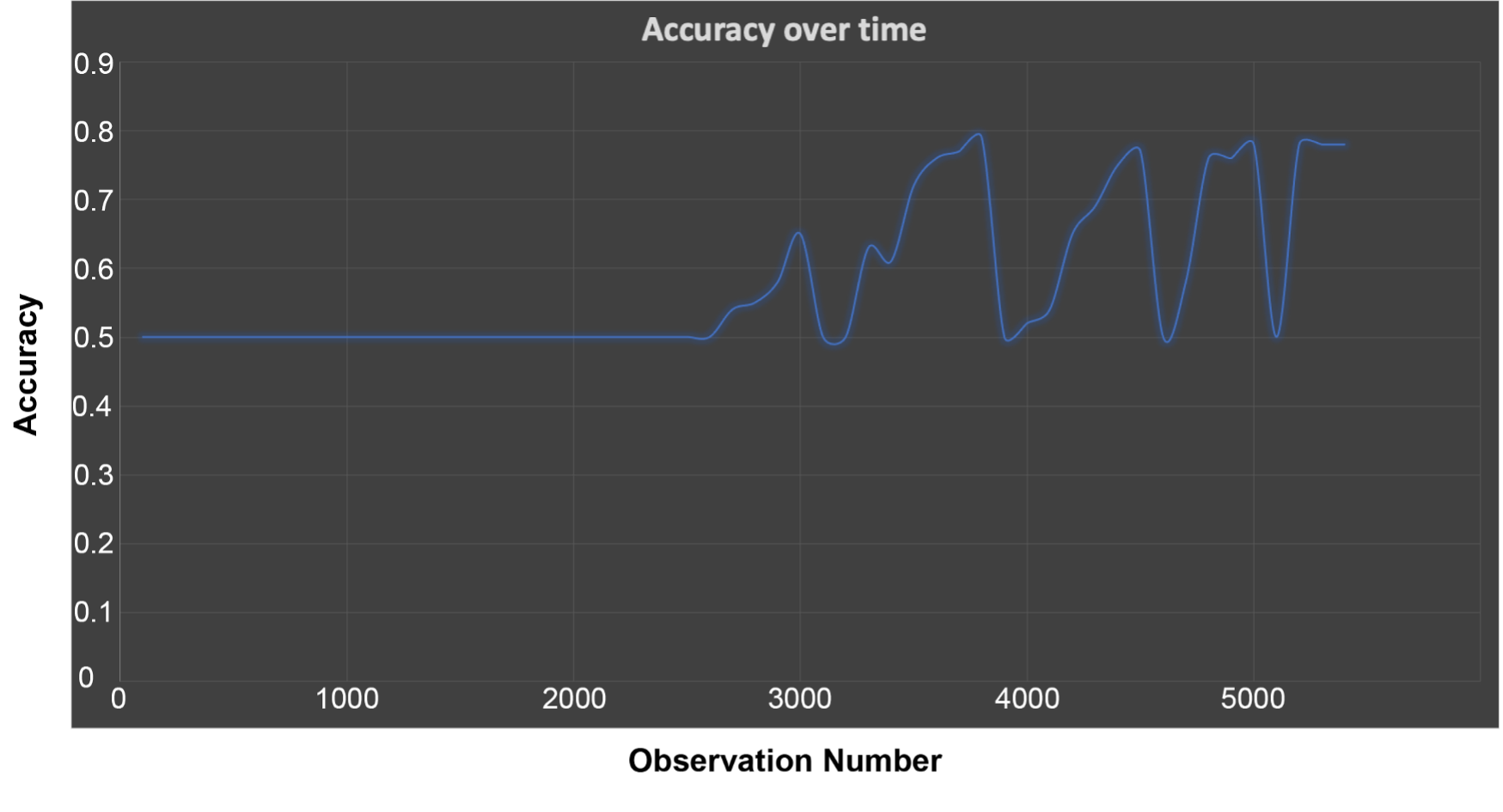
The graph shows that the accuracy starts out as no better than guessing (0.5) initially, as expected, as incremental training starts off with no data. It takes a long while to improve from this base state, and then oscillates wildly up and down between 0.5 and 0.8. This is slightly alarming, as it will be just a matter of luck if the model is better than guessing or not at any point in time during the training—and for incremental learning, as training is continuous, this is anytime in practice.
What can be done about this? A constraint with incremental learning is that we are trying to update the model from the most recent data. But it looks like we are getting stuck in a local minima due to the use of a very small batch consisting of just the latest data for training for each increment, so normal solutions such as shuffling the data doesn’t help much. A possible solution is to checkpoint/save the model when the accuracy reaches some threshold, e.g., above 0.7 accuracy. Then continue to use the saved model for prediction until a better one comes along.
3. Predictions

Zoltar Speaks—would you like a prediction of your future? (Photo by Robert Linder on Unsplash)
And talking about prediction, how would prediction work in practice for this example? The idea behind learning (of any approach) is to be able predict the class of (as yet) unseen future events. For our drone delivery shop busy/not busy model, the idea therefore is to be able to use it warn shops if they will be busy ahead of time, so that they can prepare in advance. After a week of learning, we may feel confident to predict which shops will be busy in the opening hour of deliveries for the next week. We can simulate this by predicting on the first hour of data from our existing dataset using the following code:
|
1 2 3 4 5 6 7 8 9 |
print("predict on Monday hour 1 data...") res = model.predict(drone_features[0:99]) for r in res: for v in r: print(v) |
This prints out a list of values from 0 to 1.0. I was surprised that they are all decimal numbers, not the expected integer 0 or 1 representing the binary classes. I concluded that the numbers represent the probability of the class being 0 or 1—the higher the value the more likely it is that the class is 1. So, I introduced round(v) to either round up or down to produce 0 or 1’s (What happens if you are dealing with a multiclass learning problem I wonder? Apparently the softmax function—more about that here – is your friend). Comparing the predictions to the actual classes resulted in an accuracy of 0.75.
However, I also thought of another approach. What if you don’t make predictions for more uncertain results? For example, by only making a prediction if the prediction is <= 0.2 or >= 0.8, the predictive accuracy improved to 0.9, although at the cost of not making a prediction for 26% of the shops. Here’s the final code:
|
1 2 3 4 5 6 7 8 9 10 11 |
for r in res: for v in r: if v <= 0.2 or v >= 0.8: print(round(v)) else: print("-1") |
I also thought of another complication with prediction—one of my own creation, unfortunately. Apart from the features that are actually relevant for the busy/not busy rules, I introduced some other features just to make it a bit more realistic (e.g., average delivery time, customer rating, etc.). However, the values of these features are not known until the end of each hour, so cannot be part of the data being predicted over. And the data to predict over must be the same shape as the training data—so you can’t just drop features. Also, with neural network models, I suspect that you can’t tell what features are actually being used by the model. What’s the solution? Potentially replacing them with “average” values.
4. Conclusions
With careful tuning of some settings (sample size, batch size, fixed epochs), incremental training with TensorFlow can produce models that are comparable with batch training, and the training time is similar. However, there are a couple of things to watch out for, including that the incrementally trained model doesn’t exhibit continuous incremental improvement in accuracy, but rather wild oscillations in accuracy. For a production environment, more accurate models may need to be checkpointed and used instead of the current model for prediction if accuracy drops. So, you may end up having to manage multiple models—based on some initial experiments I’ve done, this trick may also be useful for data with concept drifts potentially. You will also need to constrain the growth of the evaluation data set size (which with streaming data will just keep growing otherwise), e.g., use the last 10,000 samples etc.
I also still worry about the use of all the data for training as this can result in overfitting—in theory sampling from streaming data could work. And this may also help with another potential issue, which is how to keep up with the training on a data stream with increasing volumes.
At some point the incremental training will start taking longer than the time between polls, so one solution is to reduce the number of samples dynamically to ensure it keeps up. Another approach may be to run distributed training (or even train multiple models based on what partitions each Kafka consumer is mapped to). The opposite problem is related to low throughput data: what if there’s insufficient data available each poll? Then you probably need to cache/aggregate the data until you get 100 samples to train on.
Next blog we’ll connect our incremental TensorFlow code up to Kafka and see how it works.
Acknowledgements
Thanks to some of my colleagues who turned out to be secret ML gurus, for providing feedback so far during this blog series, including Justin Weng and Nikunj Sura.
Follow the series: Machine Learning Over Streaming Kafka® Data
Part 2: Introduction to Batch Training and TensorFlow
Part 3: Introduction to Batch Training and TensorFlow Results
Part 4: Introduction to Incremental Training With TensorFlow
Part 5: Incremental TensorFlow Training With Kafka Data
Part 6: Incremental TensorFlow Training With Kafka Data and Concept Drift