Machine Learning Over Streaming Kafka Data

Dev Rel
Apache Kafka
Technical

Machine Learning Over Streaming Kafka Data—Part 6: Incremental TensorFlow Training With Kafka Data and Concept Drift

October 17, 2023
By Paul Brebner

In the “Machine Learning over Streaming Kafka Data” blog series we’ve been learning all about Kafka Machine Learning—incrementally! In the previous part, we connected TensorFlow to Kafka and explored how incremental learning works in practice with moving data. In this part, we introduce concept drift, try and reduce noise, and remove time!

1. Concept Drift

Snow drifts may come as an unexpected surprise (Source: Shutterstock)

1.1 The Same Model for 2 Weeks

One of the main use cases for incremental/online training is when there’s a change in the world and the data also changes to reflect it. For the next experiment, I changed the rules for shop busy/not busy but kept the distribution the same (approximately 50% busy), and the change was for the entire 2^nd week (across all days). Using the incremental training, we, therefore, expect the model to be surprised and perform worse at the start of the 2^nd week of data, but then to (hopefully) improve again – although by how much is anyone’s guess Even with incremental learning, the model doesn’t forget, so it will still be trained with the 1^st week of data while trying to learn the 2^nd week as well.

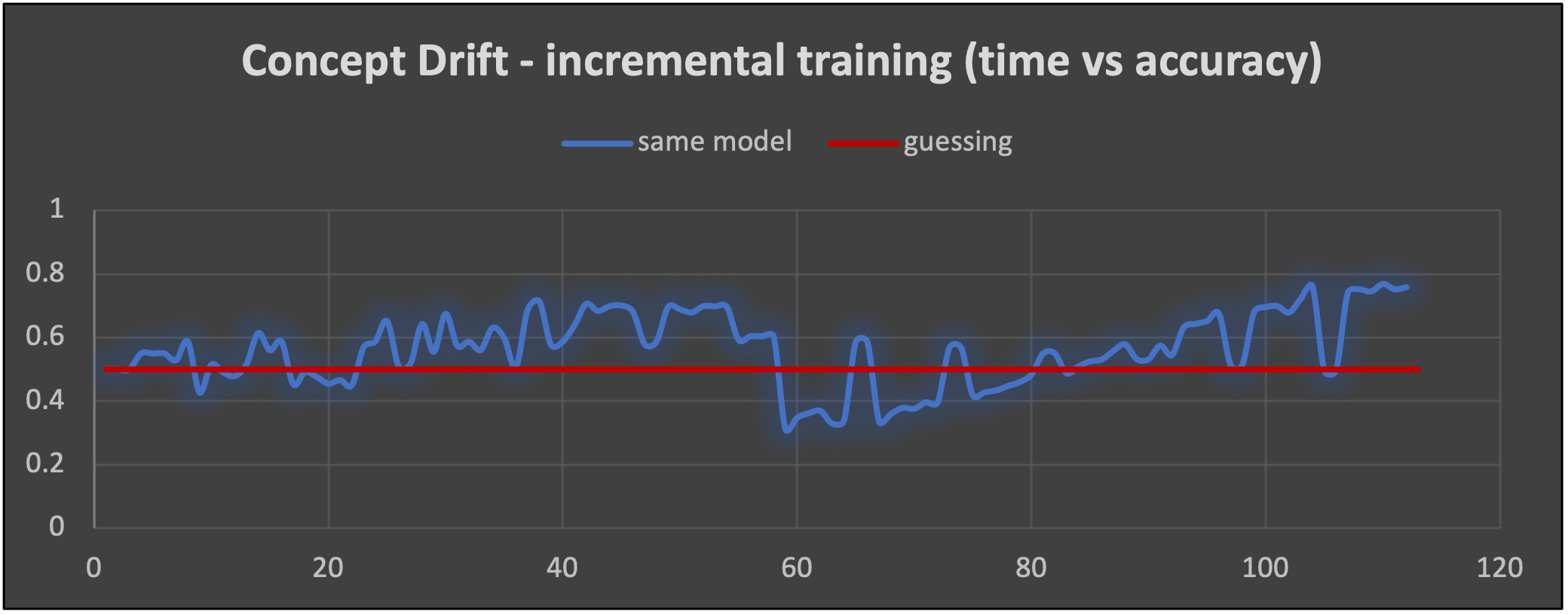
For the 1^st week of data, the incremental model shows the typical oscillation but does improve over time, reaching a maximum accuracy of around 0.7. When it encounters the 2^nd week of data, which has the concept drift, the accuracy instantly drops below the 0.5 “guessing” line. The model is still obviously dominated by the training from the (now different) 1^st week of data, so is performing worse than guessing initially, but the impact of the newer training (and evaluation) data does seem to gradually kick in and the accuracy peaks at a better 0.75.

1.2 A Different Model for Week 2

What can we do differently and maybe better? One obvious tactic to try is to detect a sudden drop in the model accuracy, assume that we’ve encountered a concept drift, and just start training from scratch again (in my case I did this by recompiling the model). Here’s the extra code (highlighted) added to the training loop, in practice you would need a more sophisticated approach to trigger the model reset than just a simple drop in accuracy:

if l > 0:

model.fit(train_mini_ds, batch_size=BATCH_SIZE, epochs=EPOCHS)  
  	res = model.evaluate(test_mini_ds)
  	last_acc = res[1]
  	accs.append(last_acc)
  	print("accuracy = ", last_acc)
  	if last_acc > best_acc:
  		best_acc = last_acc
	if last_acc < 0.4:
  	    print("Reset model!")
  	    model.compile(optimizer=OPTIMIZER, loss=LOSS, metrics=METRICS)
  	    model.fit(train_mini_ds, batch_size=BATCH_SIZE, epochs=EPOCHS)
  	    test_mini_ds = mini_ds.skip(80)
  	    res = model.evaluate(test_mini_ds)
  	    last_acc = res[1]
  	    accs.append(last_acc)
  	    print("accuracy = ", last_acc)
                 best_acc = last_acc

model.fit(train_mini_ds, batch_size=BATCH_SIZE, epochs=EPOCHS)

res = model.evaluate(test_mini_ds)

last_acc = res[1]

accs.append(last_acc)

print("accuracy = ", last_acc)

if last_acc > best_acc:

best_acc = last_acc

if last_acc < 0.4:

print("Reset model!")

model.compile(optimizer=OPTIMIZER, loss=LOSS, metrics=METRICS)

model.fit(train_mini_ds, batch_size=BATCH_SIZE, epochs=EPOCHS)

test_mini_ds = mini_ds.skip(80)

res = model.evaluate(test_mini_ds)

last_acc = res[1]

accs.append(last_acc)

print("accuracy = ", last_acc)

best_acc = last_acc

The results from this approach are surprising (orange graph below).

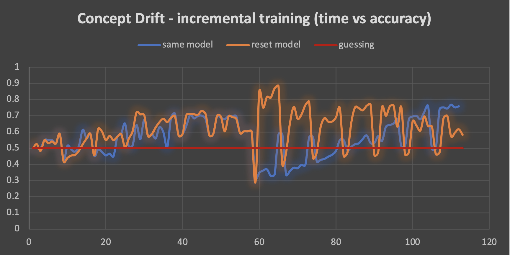
This time the reset model must start from scratch with the 2nd week of data. Surprisingly this actually helps it briefly, as the accuracy momentarily leaps to 0.9, but then drops and oscillates as is more normal for incremental learning. By the end of the 2nd week, the best accuracy is around 0.7.

2. More Data = Less Noise?

Maybe we need some noise cancellation too! (Source: Shutterstock)

The oscillation of the accuracy of the incremental model is an obvious issue. The period of oscillation also appears to be regular and looks suspiciously correlated with something about the data. The obvious conclusion to draw is that it’s related to the days of the week. Given that the data contains time features—day of week and hour of day—it’s possible that the model is overfitting on these. And the evaluation accuracy may be dropping because some hours of the day have no busy shops. Maybe we also just don’t have sufficient data. More data is a well-known solution for reducing the impact of noise on ML.

I created a 2^nd test data set to try and overcome some of these problems. I changed the rules so that every delivery is now an observation, and the class represents if the delivery is delayed or not delayed by more than the average delivery time (but using the busy/not busy shop rule still). I also replaced the weekday feature (as it’s a potential source of noise) with a 0 value so it would be ignored. The test data now has 2000 observations per hour, giving over 100,000 records for a week (compared to 5599 observations per week for the original data set). There’s no concept drift in this data at present. Here are the incremental learning results over the larger week data set:

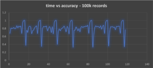
We are still getting the oscillation (as the data still contains day hours), and the swing is bigger—from 0.5 to 1.0. For comparison, I also ran the batch training on the same data. The accuracy on the training data was 0.9568, and 0.74 on the evaluation data.

Given the increase in data size, I also increased the Kafka consumer polling batch size to 1000. However, I noticed that this resulted in the consumer timing out it was taking longer than 10s (the timeout period) to fit each time. This is a good example of the “slow Kafka consumer” problem—and would need to be addressed in a production Kafka+ML system (for more information see some previous blogs, and the new Kafka parallel consumer blog series coming soon).

For both the incremental and batch training, the model does better on the training data than the test set, so overfitting is likely the problem. This seems to be a well-known issue with learning over timeseries data, so I won’t try and improve it for the time being. Here are some useful references:

Basically, timeseries machine learning is tricky! So, let’s get rid of time!

3. No Time Features

Time to try “no time” (Source: Shutterstock)

For the final experiment I tried new rules and data with no time feature dependencies, just distance, shop type, and location. I generated 2 weeks of the small data set again, with a change in the rules for the 2nd week to include concept drift. Here are the results:

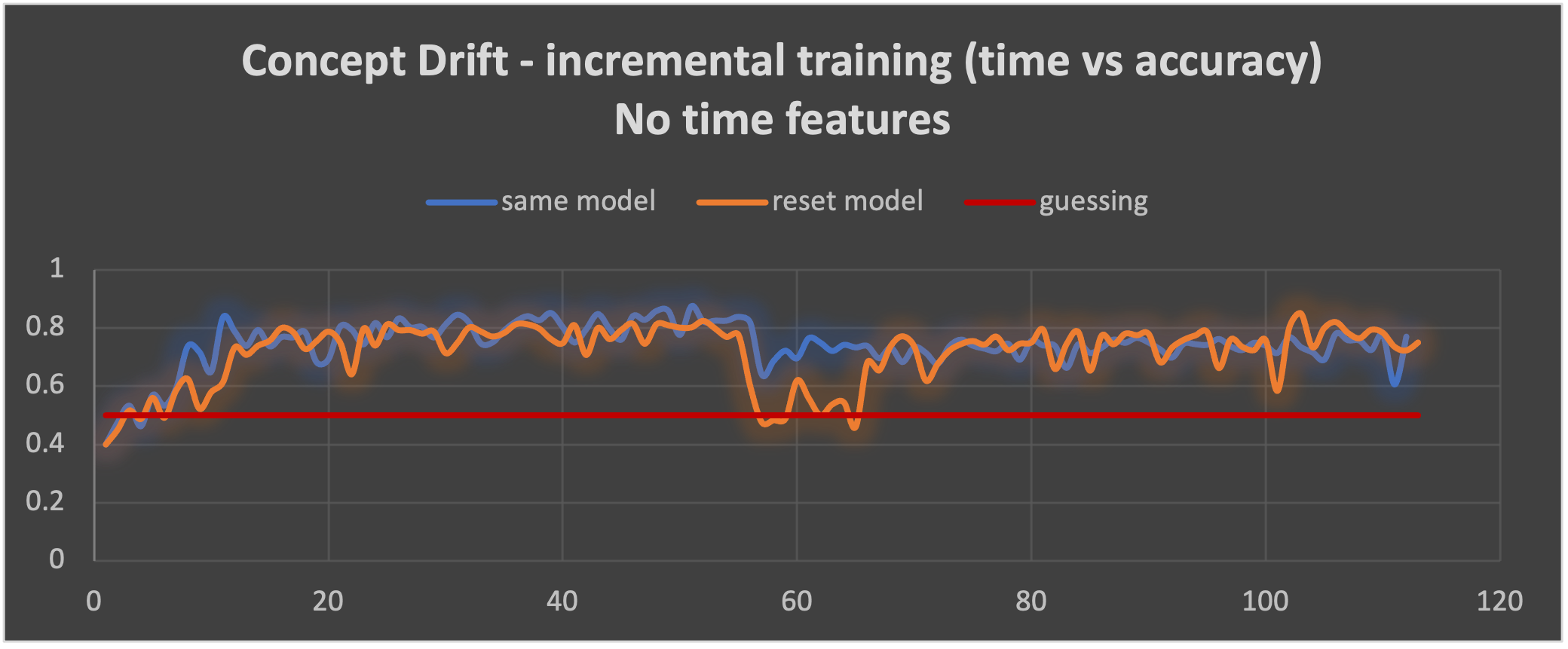
It does look like we’ve finally succeeded in removing the wild oscillations, so our theory that they were related to the time features in the data and rules is validated. The incremental model with no reset (the blue line) shows a rapid improvement in accuracy up to over 0.8 accuracy for the 1^st week of data (best accuracy of 0.875). When the concept shift occurs, there is a consistent drop in accuracy to around 0.75 for the remainder of the 2^nd week of data. The orange line shows incremental learning with a model reset at the start of the 2^nd week of data. Resetting the model results in a substantial drop in accuracy back to the baseline 0.5 for a short period of time, then the accuracy improves again up to around 0.8 with a maximum of 0.85.

There does appear to be a difference in the 2 approaches. Not resetting the model means the model trained on the 1^st week of data struggles to relearn for the 2^nd week of data and does not perform as well. But at least there’s no big drop in accuracy which is observed when we reset the model and start learning from scratch again. A workaround for this could be to continue using the original model for predictions until the new model has comparable accuracy, and then switch over to the new model. Resetting the model does eventually result in better accuracy over the new 2^nd week of data, so it may be a better tactic to cope with concept drift.

4. Observations

(Source: Shutterstock)

Given our incremental approach to Kafka incremental machine learning, it’s taken a while to get here. However, incremental learning with TensorFlow over Apache Kafka data is practical, even with the basic TensorFlow Kafka framework. For use in production, there will be a number of things to watch for, including:

How best to construct a model and the choice of hyperparameters
How to tune the incremental learning including epochs, and all the different “batch” sizes
How to select training and validation data
How to design the topics/partition/keys for the data (for training, evaluation, and prediction)
If and when to reset the model and start from scratch again
What to do if there’s too much oscillation in the accuracy of the model (potentially due to time-based features)
How to apply the model for prediction over Kafka data (and if to use more than one model)
And finally, how to achieve scalability of training with increased streaming data volume—even incremental training takes time, and you may need to train multiple concurrent models or one model using distributed training to achieve real-time Kafka ML. In future parts of this series, we’ll explore some other frameworks that may make this task easier.