ApacheCon@Home is over for 2020 and was a resounding success, with close to 6,000 attendees from every continent. As a Platinum Sponsor, Instaclustr ran an ApacheCon Booth and this blog was originally presented on 30 September 2020 as a booth talk.

I was one of the 1% attending from Australasia:

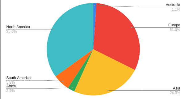
This, unfortunately, meant I was seriously spatiotemporally challenged, as Pacific Daylight Time, the ApacheCon timezone, is 17 hours behind Australian Eastern Standard Time. But even though I was out of sync, at least I was ahead (see why the rotation of planets is relevant for the use case below). I also didn’t get to watch any of the other interesting ApacheCon talks in real-time this year, but I did present two talks (the other was in the geospatial track) at around sunrise in Australia, not a sight that I normally behold.

1. Why These Technologies?

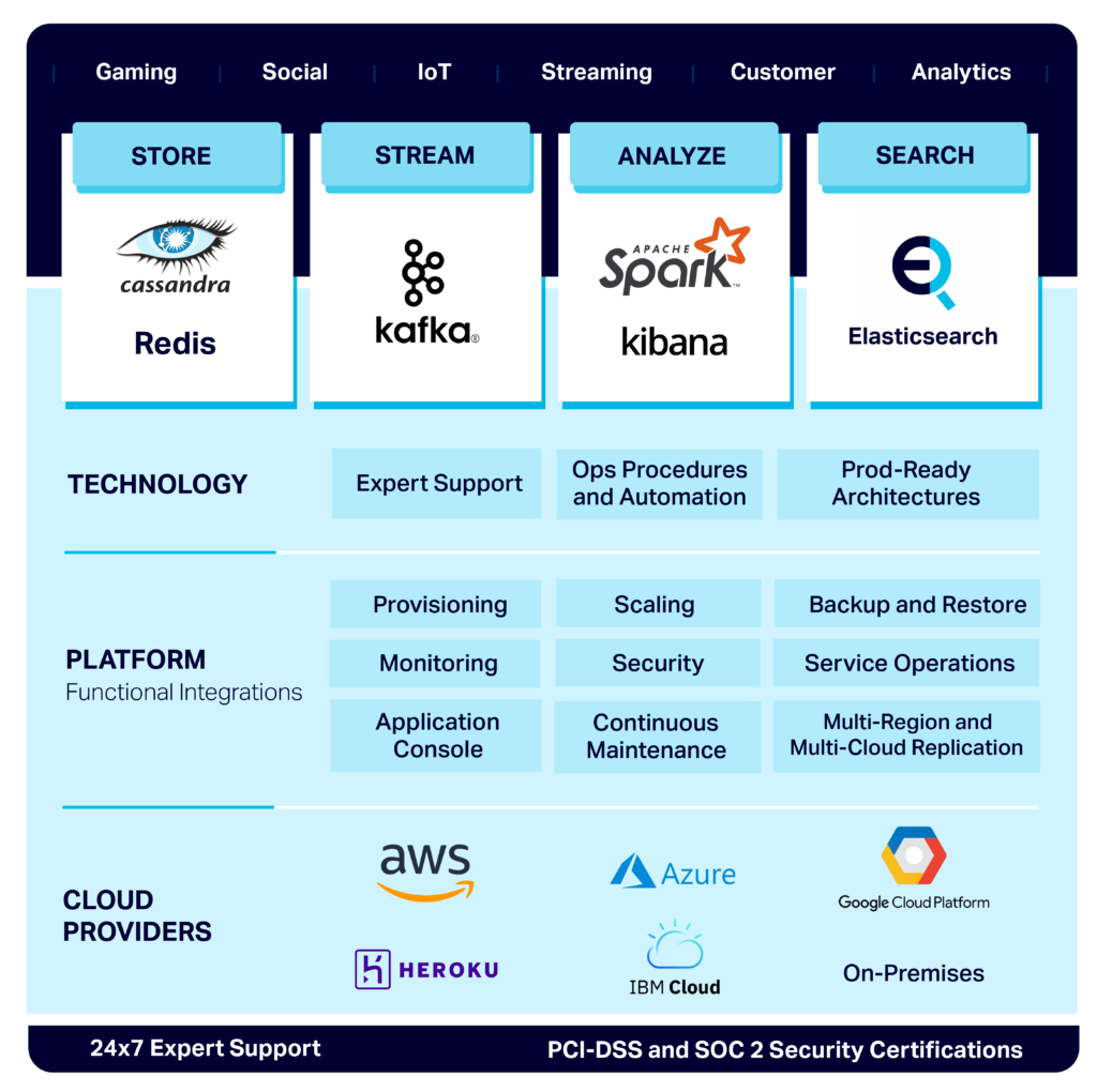
If you’ve read any of my previous blogs you’ll know that I’m the technology evangelist for Instaclustr. Instaclustr offers the Instaclustr Managed Platform, which is a complete ecosystem to support mission critical Open Source Big Data applications. We currently have managed Cassandra and Redis (for storage), Kafka and Kafka Connect (for streaming and integration), Spark and Kibana (for analytics and visualization), and Elasticsearch (for Search). Our platform supports provisioning, monitoring, an easy to use GUI console, scaling, security, maintenance, backup and restore, service operations, and multi-region/multi-cloud replication, on multiple cloud providers (AWS, Heroku, Azure, IBM Cloud, GGP), and on-premises:

We will focus on three recent additions to our managed platform: Kafka Connect, Elasticsearch, and Kibana.  Why did I pick these three technologies? Well, in general, the integration of non-standards based heterogeneous technologies can be complicated! “Rube Golberg” contraptions were “devices that performed simple tasks in indirect convoluted ways”!

Instead, what we need is a contraption that performs a difficult task (integration) in an easy way!

2. Integration Is Easy With Kafka Connect

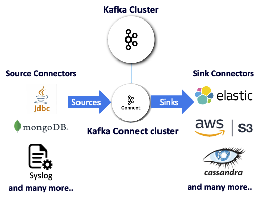
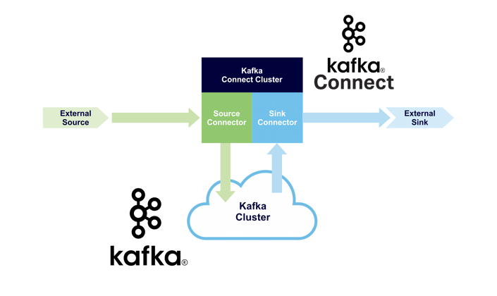
Luckily one of our target technologies, Kafka Connect, is designed to make integration easy. It’s a distributed (for high availability and scalability) solution to integrate Kafka with multiple heterogeneous data sources and/or sinks. It enables connectors (source or sink) to handle the specifics of particular integrations. Source connectors handle retrieving data from non-Kafka source technologies and sending it to Kafka topics. Sink connectors handle reading data from Kafka topics and sending it to non-Kafka sink technologies. Why use Kafka Connect? It provides zero-code integration, high availability, and elastic scaling independent of Kafka clusters. 

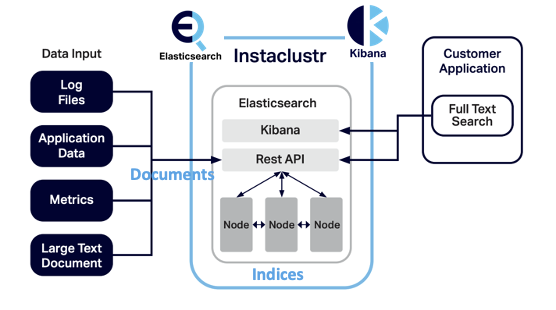
But what are we going to integrate with Kafka Connect? There are many options, only limited by your imagination and the availability of a robust Open Source Kafka Connector (or you can write your own).  For example, Elasticsearch is an obvious target sink technology to enable scalable search of indexed Kafka records, with Kibana for visualization of the results (with many graph types, and maps as well).  Instaclustr provides a fully-managed Open Distro for Elasticsearch (100% Apache 2.0 licensed). Elasticsearch can be used to index and search many different document types, and in this blog, we’ll demonstrate the integration between real-time streaming data and Elasticsearch using Kafka Connect.

3. What’s the Story?

Once Upon A Time (several months before ApacheCon @Home 2020), I attended the 2020 Kafka Summit, where I was inspired to blog about several striking Kafka use cases and Kafka technology trends.  One of the use cases that was particularly topical was how the US Centers for Disease Control and Prevention (CDC) built a COVID-19 specific pipeline in under 30 days (Flattening the Curve with Kafka, by Rishi Tarar), resulting in this now widely recognized visualization on the CDC website: https://covid.cdc.gov/covid-data-tracker/

Apache Kafka was the obvious choice of technology, and enabled them to receive COVIDtesting data in real-time from multiple locations, formats, and protocols; integrate, and then process the raw events into high quality multiple consumable results; with appropriate data governance in place to ensure the results were both timely and trustworthy. 

Counting down to my ApacheCon@Home presentation deadline I realized I also had around 30 days to build a demo and write a talk about it. Coincidentally, one of the Instaclustr consultants (Mussa) had already built an integration demo using public data (COVID-19 and climate change batch data) via Kafka connect REST source connectors running on Docker. I thought it would be a fun challenge to go two steps further by using public streaming data, and deploying and running everything on the Instaclustr managed platform. 

So the hunt was on for suitable public streaming REST APIs, with easy to use JSON format, complete data (including position data for mapping), from an “interesting” domain, and which wasn’t political or apocalyptic in nature!  This may sound like an impossible combination, but after a few false starts, I finally settled on a domain which is reassuringly outside the scope of human impact (or so I thought)—Tides!

4. The Lunar Day and Tides

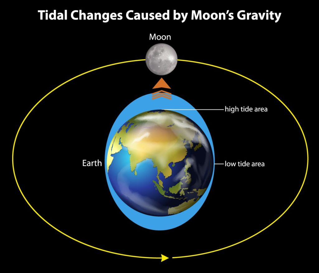
I always had a vague notion that tides don’t exactly follow the Earth Day (a complete rotation, taking 24 hours). But did you know that they actually follow the “Lunar Day”? This is the period between moonrises at a particular location on the Earth, possibly better called the “Tidal Day” due to likely confusion with the length of a day on the moon (which is the more familiar 29.5 Earth days). Confused? This simple explanation of Tides from the NOAA website will help:

Unlike a 24-hour solar day, a lunar day lasts 24 hours and 50 minutes. This occurs because the moon revolves around the Earth in the same direction that the Earth is rotating on its axis. Therefore, it takes the Earth an extra 50 minutes to “catch up” to the moon. Since the Earth rotates through two tidal “bulges” every lunar day, we experience two high and two low tides every 24 hours and 50 minutes.

Here’s a simple picture which shows the gravitational force of the moon causing a high tide next to the moon (and another high tide on the opposite side of the Earth) every lunar day (the yellow path):

All of which makes more sense after watching this animation a few times (from the same site):

NOAA has a REST API for retrieving data from all of their tidal stations which seemed to satisfy all my requirements. And they have a “bonus” map so you can located all the stations and drill down for more details:

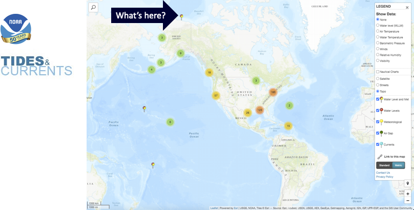
I was curious to see what was on the northernmost point of Alaska? Evidently, a place called Prudhoe Bay.

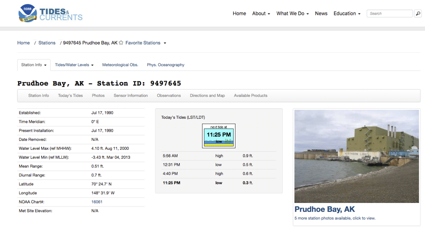
You can get detailed sensor information.

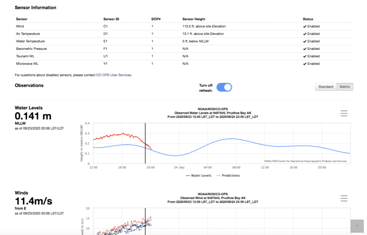
Here’s an example REST call including station ID, data type and datum (I used water level, and mean sea level), and a request for just a single/latest result with metric units:

https://api.tidesandcurrents.noaa.gov/api/prod/datagetter?date=latest&station=8724580&product=water_level&datum=msl&units
=metric&time_zone=gmt&application=instaclustr&format=json

Which returns this JSON result which includes lat/lon, time, and the value of the water level (Unfortunately to know what the data type, datum, and units of the result are, you have to remember what the call was!):

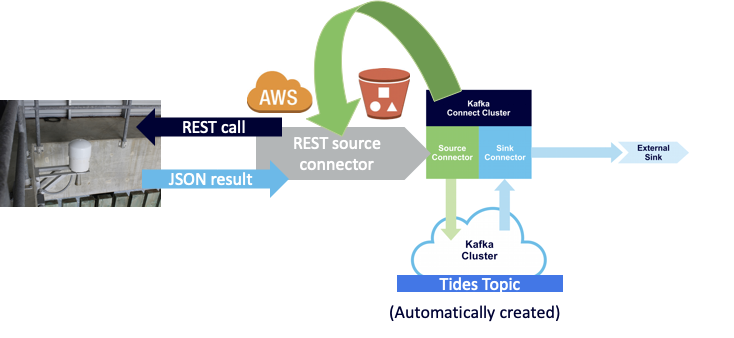
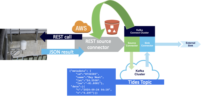
5. Start the Pipeline With a REST Source Connector

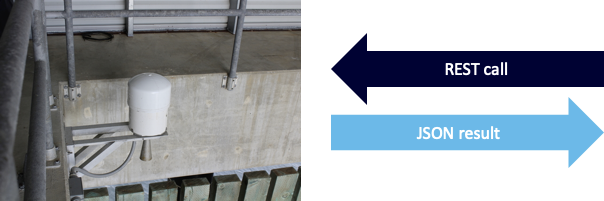
Let’s start our pipeline using this REST API for the streaming tidal JSON data source (this device is the actual water level measuring sensor, it is able to measure the water height without actually being in the water, using microwaves or similar).

What else do we need? To start with, a Kafka and Kafka Connect cluster. The easiest way to provision these on AWS is using Instaclustr Managed Kafka and Managed Kafka Connect using the Instaclustr console. The console gives you the option to select the technology, cloud provider, region, instance size, and number, and security options etc. For Kafka Connect you also specify which Kafka cluster to use. Within a few minutes you have running clusters.

Now we have a Kafka cluster and a Kafka connect cluster available for use.

Next, find a REST connector (I used this Open Source REST connector), deploy it to an AWS S3 bucket (here are the instructions for uploading connectors to a S3 bucket), tell the Kafka connect cluster which bucket to use, sync so it’s visible in the cluster, and then we are ready to configure the connector and run it. Instaclustr calls this feature “BYO connector”, which means you are not locked into a finite set of connectors that may not be suitable for your requirements. 

Because the Instaclustr managed Kafka connect is pure open source, the connector configuration is done in the standard Kafka connect way using a REST API. Here’s an example using “curl”, which includes the connector name, class, URL, and topic (you will need to change the URL, name and password details):

This creates a single connector task which polls the REST API every 10 minutes, and writes the result to a Kafka topic, “tides-topic”. I picked five random tidal sensors to use, so I ended up with 5 different configurations and 5 connectors and tasks running. Now we have tidal data coming into the tides topic… What next?

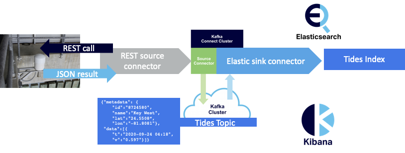
6. End the Pipeline With an Elasticsearch Sink Connector

Next, we need somewhere to put the data, so I provisioned a managed Elasticsearch cluster with managed Kibana using the Instaclustr console. Within a few minutes, the cluster is available, and now we just need to configure the included open source Elasticsearch sink connector to send data to Elasticsearch.

Here’s an example configuration showing the sink name, class, Elasticsearch index and Kafka topic. The index is created with default mappings if it doesn’t already exist.

Great, it’s all working! Sort of… Tide data is arriving in the Tides index. 

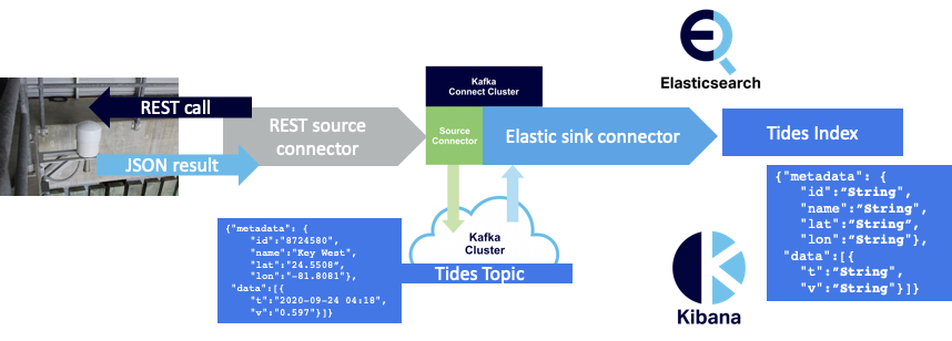
But, using default index mappings, everything is a String. To graph time series data correctly in Elasticsearch (i.e. time on the x-axis in order, and the value on the y-axis) we need a custom mapping instead. Here’s how to create a custom mapping for the tides-index with the JSON “t” field as a custom date (the date doesn’t have seconds), “v” as a double, and “name” as a keyword (for aggregation):

Welcome to Elasticsearch “reindexing”. Every time you (1) change an Elasticsearch index mapping you typically have to (2) delete the index, (3) reindex all the data again. But where does the data come from? There are two options. As we are using a Kafka sink connector, all of the data is already in the Kafka topic, so you can just replay it. Or, you can use the Elasticsearch reindex operation. 

7. Graph Visualization With Kibana

Because we are using the Instaclustr Managed Platform we can just start Kibana with a single click in the Instaclustr console as shown by the hand in this screenshot:

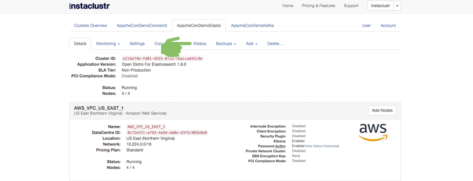
Which takes you to this Kibana home screen. We are now just three steps away from creating a simple visualization of the tidal data as follows:

1. Create an Index Pattern (to get data from Elasticsearch)
   • Settings -> Index Patterns -> Create Index Pattern -> Define -> Configure with “t” as timefilter field
2. Create Visualization (to create a graph type)
   • Visualizations -> Create Visualization -> New Visualization -> Line -> Choose Source = pattern from (1)
3. Configure Graph Settings (to display data correctly)
   • Select time range, select aggregation for y-axis = average -> data.v -> select Buckets -> Split series metadata.name -> X-axis -> Data Histogram = data

Which results in this nice graph showing the tidal data over time (time on x-axis; tide level, relative to average level, in meters) for the 5 sample stations (averaged over 30 minutes):

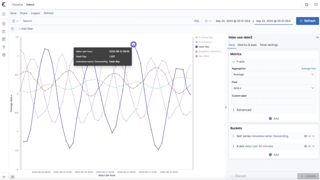
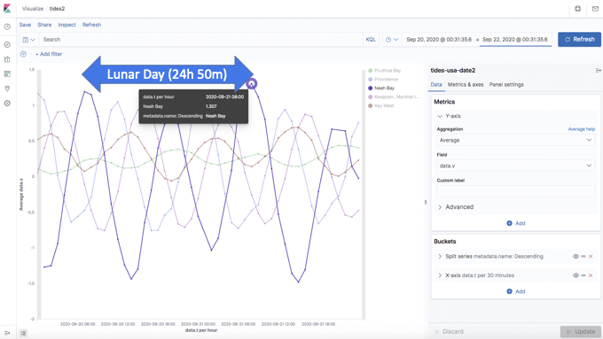
This is cool as it reveals a couple of interesting things about the tidal data that we wouldn’t otherwise have seen from the raw data. First, it clearly shows that tides are periodic, and that the period of time between two consecutive high tide peaks is the Lunar Day (24 hours and 50 minutes):

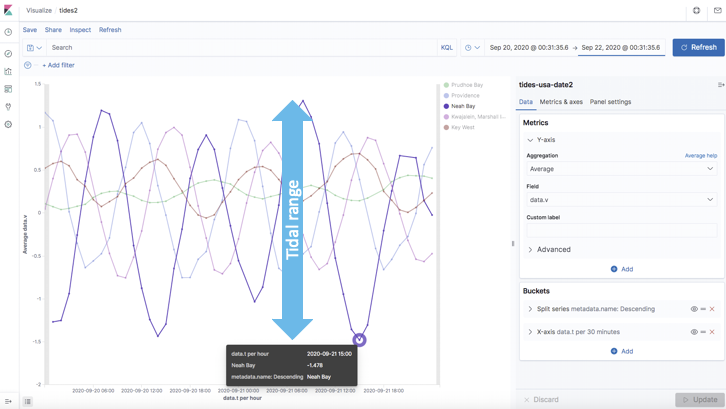
Slightly more unexpected, it also shows that the Tidal Range (difference between high and low tides) is different in all of the locations. For example, the tidal range at Neah Bay is close to 3 meters, which is a lot more than the smallest range (Prudhoe Bay, < 0.5 meters).

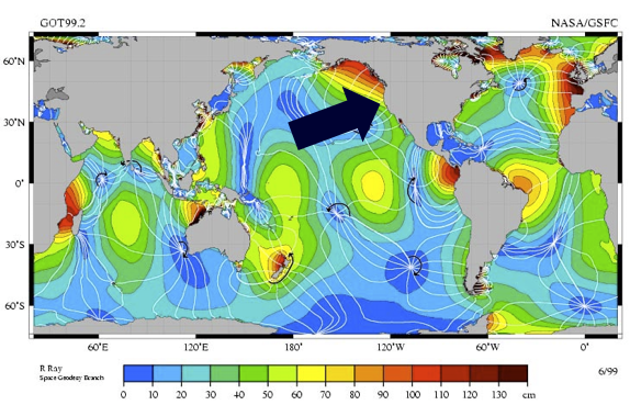
Why is this? Well, it turns out that tide range varies depending on the Moon, the Sun, local geography, weather, and increasingly, climate change. So my guess that Tidal data was a “safe” domain was only half correct, as the tidal period is invariant, but the tidal range is increasingly higher and more unpredictable due to rising sea levels, and weather anomalies including storm surge flooding.

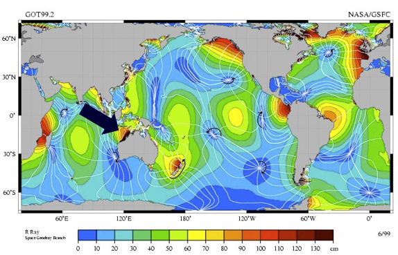
This map of the world shows tidal hotspots in red, with the arrow point to Neah Bay (close to a hotspot):

Australia’s biggest tidal hotspot is here, in the Kimberley’s. 

Tides of over 11 meters are forced through two narrow passes creating the popular tourist attraction known as the Horizontal Waterfalls in the Kimberley’s Talbot Bay.

8. Mapping Data in Kibana

Given that the tidal data sensors are at given geospatial locations, and the lat/lon data is in the JSON already, it would be nice to visualize the data on a Kibana map. But, at the first attempt, nothing appeared on the map. 

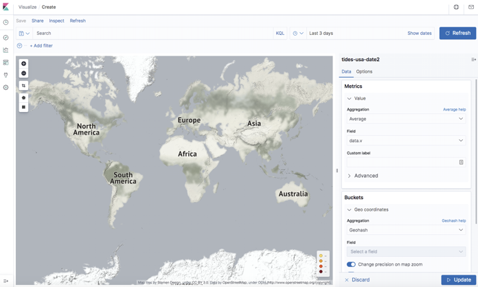
Why not? Find out why and a solution in part 2 of this blog.

Follow the Pipeline Series

• Part 1: Building a Real-Time Tide Data Processing Pipeline: Using Apache Kafka, Kafka Connect, Elasticsearch, and Kibana
• Part 2: Building a Real-Time Tide Data Processing Pipeline: Using Apache Kafka, Kafka Connect, Elasticsearch, and Kibana
• Part 3: Getting to Know Apache Camel Kafka Connectors
• Part 4: Monitoring Kafka Connect Pipeline Metrics with Prometheus
• Part 5: Scaling Kafka Connect Streaming Data Processing
• Part 6: Streaming JSON Data Into PostgreSQL Using Open Source Kafka Sink Connectors
• Part 7: Using Apache Superset to Visualize PostgreSQL JSON Data
• Part 8: Kafka Connect Elasticsearch vs. PostgreSQL Pipelines: Initial Performance Results
• Part 9: Kafka Connect and Elasticsearch vs. PostgreSQL Pipelines: Final Performance Results
• Part 10: Comparison of Apache Kafka Connect, Plus Elasticsearch/Kibana vs. PostgreSQL/Apache Superset Pipelines