In Part 3 of this blog series, we looked at Apache Camel Kafka Connector to see if it is more or less robust than the connectors we tried in Part 1 and Part 2. Now we start exploring Kafka Connect task scaling. In this blog we will:

• Change the data source so we can easily increase the load 
• Select some relevant metrics to monitor, and work out how to monitor the end-to-end pipeline with Prometheus and Grafana

1. Monitoring and Scaling (Camel) Kafka Connector Tasks

What’s better than one camel? Lots of camels (potentially). Just as a camel train is the best way of transporting lots of goods long distances in the desert, multiple Kafka Connector tasks are the way of achieving a high throughput data pipeline:

But you also don’t want too many! It turns out that the introduced camels liked the Australian outback so much that we now have the largest wild camel herds in the world (more than one million Camels). In this blog, we’ll explore how to best manage the population of (Camel) Kafka Connector tasks.

So far in this blog series, we’ve only tried very low rate data, single connector tasks, and have focused on the functionality and robustness of the pipeline. One of the most important reasons for using Kafka connect for integration is for scalability and high throughput and buffering (complementing the availability of many different connectors, reliability, and functionality which we looked at in the last three blogs). So it’s now time to crank up the throughput and work out how to monitor and scale the number of tasks.

2. Generate Load With Kafka Source Datagen Connector

One of the constraints of using the public NOAA REST API for the input data in our pipeline is that the data is only updated every 20 minutes, and it wouldn’t be very polite to start hammering their infrastructure with hundreds or thousands of requests a second (and it may well be rate-limited). So it’s time to diverge from our Tides story in the interest of scalability.  

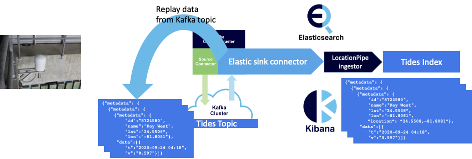
One simple way to increase the rate on the Kafka sink connector side of the system is simply to replay the data already in the Kafka records. However, this doesn’t accurately reflect all of an end-to-end pipeline (as we’ve disconnected the source side), and it’s not possible to control the rate, as the Kafka sink connector will simply read data from the topic as fast as it can. Although this is a reasonable way of finding the maximum throughput of the sink side of the system.

I remembered reading about a synthetic data/load generator for Kafka a while ago, and after some searching I found two solutions based on Kafka source connectors (both called “kafka-connect-datagen”, A and B). I tried both but ended up using the second one for further experiments. Once uploaded to an AWS S3 bucket you can resync the Instaclustr Kafka Connect cluster to recognize it as an available connector. Configuration is easy, here’s an example:

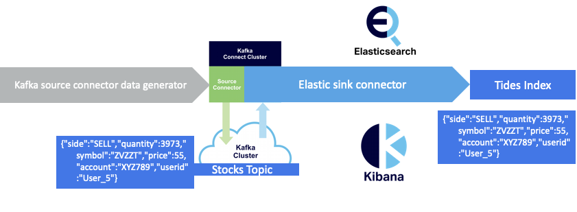
Note the change in the “story” to stocks trading (maybe Camel trading?!)—which also strengthens the “real-time” requirements as you can’t afford to wait seconds for updates to stock prices for high volume automated financial trading applications—using a “quickstart” which generates random stock tickers looking like this:

Also note the use of “price” as the keyfield. I didn’t have this initially—see Part 5 to find out why it’s necessary for scalability.

To increase the data production rate you simply decrease the “max.interval” and/or increase the number of tasks. One final thing to watch out for (if you are running long tests) is that once it reaches the maximum “iterations” the task goes into the FAILED state. This can be avoided by setting “iterations” to -1 (infinite). 

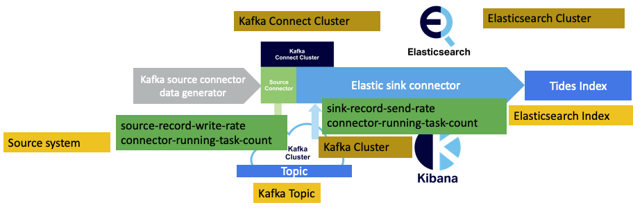
We end up with the following simplified pipeline:

 

3. Collect Metrics From Multiple Clusters With the Instaclustr Monitoring API and Prometheus

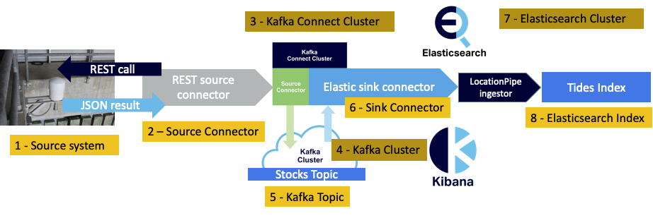
How do we do end-to-end throughput, latency, and “lag” (number of messages queued and unprocessed) monitoring of our complete pipeline, given that there are multiple systems, clusters, and components involved? Here are the potentially relevant “systems” to monitor— excluding Kibana—as we assume that the pipeline ends with the Elasticsearch indexing, even though in practice there will also be queries and visualization performed by Elasticsearch and Kibana on the indexed data:

• Source system—in this case, none, as the data generation is synthetic and running in the Kafka Connect cluster. Even if we were using the original REST source connector, the source system (REST API) would be external to our system so impossible to monitor
• Kafka source connector
• Kafka Connect cluster
• Kafka cluster
• Kafka topic(s)
• Kafka sink connector
• Elasticsearch cluster (sink system)
• Elasticsearch index (sink endpoint)

Because we are using the Instaclustr Managed Platform, all of the cluster/node-level metrics for each technology are already available on the Instaclustr console (i.e. Kafka monitoring, Kafka Connect monitoring, Elasticsearch monitoring). The cluster level metrics are useful to ensure that the hardware resources for each technology are sufficient (e.g. CPU, disk, memory), but by themselves are not sufficient to monitor end-to-end application behaviour. 

 

For that, we need to explore what’s available from the Instaclustr monitoring API for each cluster type (i.e. Kafka connect monitoring API metrics, Kafka monitoring API metrics, Elasticsearch monitoring API metrics). The key is to find the relevant metrics and those at the most useful granularity (e.g. metrics are typically available for data center, cluster, node, component, etc.). 

Let’s start with the Kafka Connect metrics. All of the possible Kafka Connect metrics are listed in the Apache Kafka Connect monitoring documentation. Searching for “rate” metrics we find the following:

Source Metrics

Source-record-poll-rate: The average per-second number of records produced/polled (before transformation) by this task belonging to the named source connector in this worker.

Source-record-write-rate: The average per-second number of records output from the transformations and written to Kafka for this task belonging to the named source connector in this worker. This is after transformations are applied and excludes any records filtered out by the transformations.

Sink Metrics

Sink-record-read-rate: The average per-second number of records read from Kafka for this task belonging to the named sink connector in this worker. This is before transformations are applied.

Sink-record-send-rate: The average per-second number of records output from the transformations and sent/put to this task belonging to the named sink connector in this worker. This is after transformations are applied and excludes any records filtered out by the transformations.

There are also corresponding “total” metrics, but these appear to be of limited value as they are reset when tasks are restarted (which is a frequent operation when you are testing and debugging connectors, but they may be valuable in a production environment).

What do we notice about these metrics? 

• They are all rate (throughput) metrics, which is exactly what we need.
• They come in pairs—there’s an “input” rate (poll rate and read rate) and an “output” rate (write rate and send rate)—depending on the connector type.
• An important subtlety to note is that the rates exclude potential connector filtering.
  • i.e. it’s possible that all the records are filtered so you could have a big input rate, and zero output rate! 
  • We’re not using filtering, so the numbers should normally match.
  • But, the one occasion where there will be a difference is for the sink connector, if there are many non-JSON error records. In which case they will be sent to the dead letter queue not to Elasticsearch.
• Finally, these metrics are per task, not per connector. This means you need to know how many tasks are running for each connector, request metrics for each task, and then sum the rates across all the tasks to get the total rate per connector. 

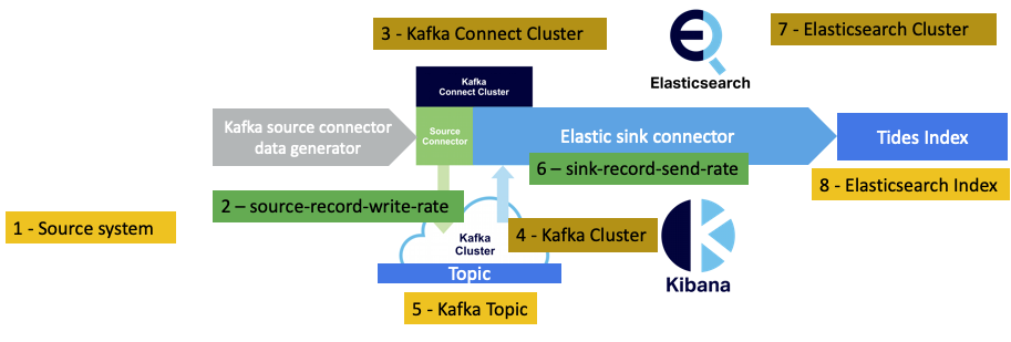
We’ll use the source-record-write-rate and sink-record-send-rate metrics as these two metrics will tell us if the sink connector tasks are keeping up with the source connector tasks. 

But are these metrics available via the Instaclustr monitoring API? If you search in the Instaclustr documentation for these exact metric names you will initially be disappointed, as the names are slightly different, and actually look like this (i.e. no hyphens, “kct” is the class of metric, “Kafka Connect Tasks”):

Also useful to monitoring is the number of running tasks for each connector, which is also available:

Connector-running-task-count: The number of running tasks of the connector on the worker.

This metric is also available via the Instaclustr monitoring API as a “Connect” Metric (“kcc”) as follows:

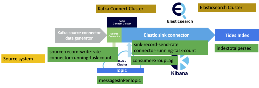
We’ll also want to keep track of the number of running tasks for both the source and sink connectors, so we now have four relevant metrics (green boxes) as follows:

It would also be useful to check that the Elasticsearch cluster is keeping up with the document indexing. There are currently a select number of Elasticsearch metrics available from the Instaclustr monitoring API, luckily including the one we need:

Note that this is the aggregate index operations per second for all the indices on the Elasticsearch cluster, so will be of limited use in production given that you will typically have multiple indices, and consequently need an index specific rate to check/tune multiple pipelines.

From the Kafka cluster, we can also get broker-level per topic metrics (“kt”), including the input rate for a topic:

kt::{topic}::messagesInPerTopic: The rate of messages received by the topic. One sub-type must be specified. Available sub-types: mean_rate: The average rate of messages received by the topic per second. one_minute_rate: The one minute rate of messages received by the topic.

We’ll want the one_minute_rate sub-type.

And finally, and also from the Kafka cluster, consumer group metrics are available, although they have a different format to the previous metrics:

consumerGroupLag: defined as the sum of consumer lag reported by all consumers within the consumer group.

Where the consumer group is the Elasticsearch sink connector, and the topic also must be specified. 

In order to be useful for end-to-end monitoring of the pipeline, all of these metrics ideally need to be displayed in once place on a single dashboard. Luckily, in previous blogs I’ve experimented with Prometheus and the Instaclustr monitoring API also supports Prometheus metrics.

Note that there is a limit of 20 metrics per request. If we run more than 20 connector tasks, then multiple requests would be needed for the task metrics, as each task counts as a metric. There is some complexity around turning the consumerGroupLag metric into a valid Prometheus configuration (the metrics path ends in kafka/consumerGroupMetrics, and extra parameters must be supplied). Cluster IDs and the monitoring API Key are obtained from the Instaclustr GUI console. Remember that the configuration must be updated whenever the number of connector tasks changes, otherwise you will be: missing values for some tasks that are running; or have metrics producing values “stuck” on the last measurement for tasks that are no longer running—both of which are confusing.

4. Prometheus and Grafana Configuration

Here’s the final prometheus.yml configuration file that I ended up with to scrape all the relevant metrics from the Instaclustr monitoring API.  This example has two source connector tasks, and five sink connector tasks.

The Instaclustr monitoring API isn’t a fully-fledged Prometheus server (just an endpoint), so to collect and display these metrics you need to set up a Prometheus server somewhere (on your local machine is fine for a demo). I also prefer to use Grafana for graphs, so you’ll also need to install it and configure a Prometheus data source. Here’s a previous blog on using Prometheus and Grafana for application monitoring in Kubernetes which covers most of the same ground. 

To display the metrics in Grafana you will need to create a dashboard with multiple graphs (I used line graphs as the data is a time series). Using the Prometheus data source, each graph has a single query. For a single pipeline, you only have to specify the basic metric name (note that the names are a bit different to those in the Prometheus configuration file), but to disambiguate the running tasks it’s best to include a tag—the name of the source and sink connectors—as follows: 

Here’s an example screenshot of the resulting dashboard (not showing the Elasticsearch index graph due to space limitations):

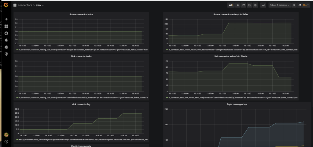
For the metrics with the [stack] annotation, you need to set “stack” ON in the visualization section of Grafana so that the corresponding graph displays the sum of all the values available. You can check that everything is working in Prometheus under the Status->Targets tab.

You can discover all the available metric names under the Prometheus graph tab (“insert metric at cursor” dropdown). However, if you have Prometheus self-monitoring enabled there will be lots of metrics to choose from. As you can see from the above metrics examples, the correct Prometheus metric name will be similar to the Instaclustr metric name (sometimes with “_” added), and it is mostly the prefix that is different. 

We’re now ready to start scaling the Kafka connector tasks in part 5 of this blog series.

Start your camels! Given the vast number of camels in Australia, it’s not surprising we have camel racing!

Follow the Pipeline Series

• Part 1: Building a Real-Time Tide Data Processing Pipeline: Using Apache Kafka, Kafka Connect, Elasticsearch, and Kibana
• Part 2: Building a Real-Time Tide Data Processing Pipeline: Using Apache Kafka, Kafka Connect, Elasticsearch, and Kibana
• Part 3: Getting to Know Apache Camel Kafka Connectors
• Part 4: Monitoring Kafka Connect Pipeline Metrics with Prometheus
• Part 5: Scaling Kafka Connect Streaming Data Processing
• Part 6: Streaming JSON Data Into PostgreSQL Using Open Source Kafka Sink Connectors
• Part 7: Using Apache Superset to Visualize PostgreSQL JSON Data
• Part 8: Kafka Connect Elasticsearch vs. PostgreSQL Pipelines: Initial Performance Results
• Part 9: Kafka Connect and Elasticsearch vs. PostgreSQL Pipelines: Final Performance Results
• Part 10: Comparison of Apache Kafka Connect, Plus Elasticsearch/Kibana vs. PostgreSQL/Apache Superset Pipelines