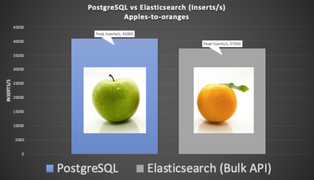
In Part 6 and Part 7 of the pipeline series we took a different path in the pipe/tunnel and explored PostgreSQL and Apache Superset, mainly from a functional perspective—how can you get JSON data into PostgreSQL from Kafka Connect, and what does it look like in Superset. In Part 8, we ran some initial load tests and found out how the capacity of the original Elasticsearch pipeline compared with the PostgreSQL variant. These results were surprising (PostgreSQL 41,000 inserts/s vs. Elasticsearch 1,800 inserts/s), so in true “MythBusters” style we had another attempt to make them more comparable.

Explosions were common on the TV show “MythBusters”!
(Source: Shutterstock)
1. Apples-to-Oranges Comparison
Next, I tried the classic “Myth Busters” second attempt methodology: just make it work! For this approach I discarded the Kafka Connect Elasticsearch sink connector and used an Elasticsearch client (The OpenSearch Python Client) directly to generate the load into Kafka (okay, this is really more like “Apples-to-weirdest fruit you can think of” comparison at this point). This client supports the security plugin, but I did have to modify it to send my example JSON tidal data, and to use the Bulk API to index multiple documents at a time.
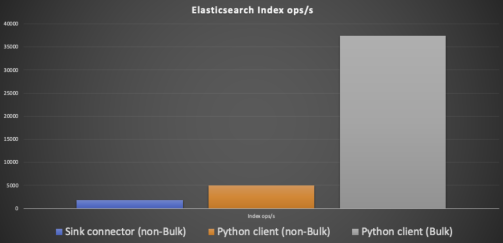
The results were definitely better this time around:
- First, using the non-Bulk API, the maximum capacity was 5,000 index operations a second (with 60 client processes, and 50% Elasticsearch data nodes CPU utilization).
- Second, using the Bulk API the maximum capacity increased to a more comparable 37,500 index operations a second (50 client processes, 80% Elasticsearch data nodes CPU, 16% master nodes CPU)
Here’s what the Elasticsearch results look like. It’s apparent that using the Bulk API makes the biggest difference, probably because the HTTP protocol is much slower than the index operation.
Now, 40,000 inserts/s translates to an impressive 3.4 billion inserts per day, way more than we would need for our example NOAA tidal data pipeline. Doing some back-of-the-envelope calculations, we have a maximum of 500 NOAA tidal stations, with 10 metrics each, refreshing every 6 minutes, so we only need 14 inserts/s. However, if the scope of our pipeline increases, say to all the NOAA land-based weather stations (30,000, and there are even more stations in the ocean and air, etc.), which have on average of say 10 metrics, and say a refresh rate every 10 seconds, then the load is a more demanding 30,500 inserts/s. Both of the prototype pipeline sink systems would cope with this load (although I haven’t taken into account the extra load on the Kafka connect cluster, due to the Kafka source connectors). This is a good example of “scalability creep”—it’s always a good idea to plan for future growth in advance.
2. Comparing Elasticsearch and PostgreSQL Replication Settings
Given my relative lack of knowledge about PostgreSQL (which is okay as we have lots of PostgreSQL experts available due to the recent acquisition of Credativ, I wondered if the replication settings for PostgreSQL were really comparable with Elasticsearch.
Elasticsearch uses synchronous replication—each index operation succeeds only after writing to the primary, and (concurrently) every replica also acknowledges it. As far as I can tell, this only happens after the write request is both written to Lucene (into memory) and to the disk log. This achieves both high durability and consistency, and the data can be immediately read from the replicas.
Here’s what I found out about PostgreSQL replication.
First, to confirm if synchronous replication is enabled (it is enabled on the Instaclustr managed PostgreSQL service, as long as you request more than 1 node at creation time), use a PostgreSQL client (e.g. psql), connect to the cluster, and run:
-
1SHOW synchronous_commit
- this will be on, and
-
1SHOW synchronous_standby_names
- which will show 1 or more node names,
- depending on how many nodes you specified at cluster creation – e.g. if 2 nodes, then there will be 1 name, if 3 nodes, then there will be 2 names
Second, “on” is the default commit mode, but there are more possibilities. Multiple options are available and include master-only or master and replicas, durability, and consistency. Here’s my summary table:
| synchronous_ commit | Commit ack when | Master durability | Replica durability | Replica consistency | Lag (increasing) |
| off | master only acks (in memory) | F | F | F | 0 |
| local | master only flush (to disk) | T | F | F | 1 |
| remote_write | replicas ack (in memory) | T | F | F | 2 |
| on (default) | replicas flush (to disk) | T | T | F | 3 |
| remote_apply | replicas applied (available for reads) | T | T | T | 4 |
The off and local modes provide no replication, whereas the rest do. All modes except off provide master durability (in the case of server failure, the data is persisted), but only on and remote_apply provide replica durability. Finally, remote_apply is the only option that also provides replica read consistency, as the data is made available for reads before the ack is sent. Note that for remote_write the data will eventually be written to disk (assuming the server hasn’t crashed – 200ms is the default time for flushes), and for remote_apply, the data will be made available for reads, but it’s just done asynchronously.
Each option will take longer to acknowledge and will in theory, therefore, reduce the throughput of the system. This also seems to be the case in practice as shown in this graph ( results normalized to best-case off mode):
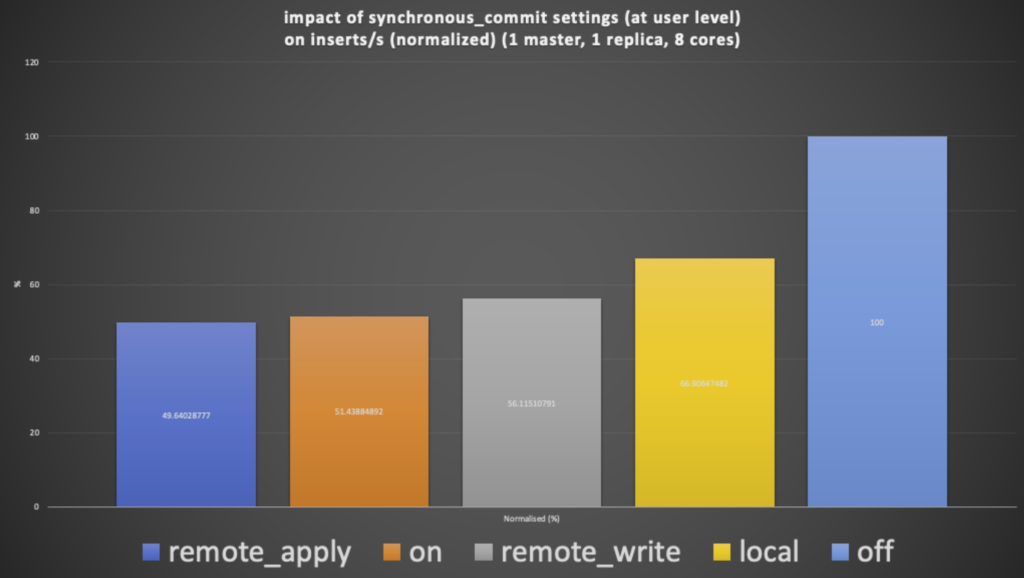
The remote_apply mode is indeed the worst case for performance, with exactly half of the throughput of the fastest off mode. So, why is this relevant for the pipeline comparison? Well, the PostgreSQL results were obtained using the default on mode. However, a more directly comparable mode, in terms of durability and consistency, is the remote_apply mode. However, in practice the performance difference between remote_apply and on is small (only about 4%) so the results are good enough for a rough comparison.
To get these results, I also had to find out how to set the scope of the settings correctly. This is because synchronous_commit can be set at the scope of transactions, sessions, users, databases, and instances (here’s a good blog to read) so I set it at the user level as follows:
|
1 |
ALTER USER username SET synchronous_commit=remote_apply; |
Finally, I was curious to see what the lags were for my running system. The best way I could find to see this was using this command:
|
1 |
select * from pg_stat_replication; |
This returns information including write_lag (corresponding to remote_write delay), flush_lag (remote_flush delay), and replay_lag (remote_apply delay), along with the sync_state of the server (which is useful confirmation that it’s working as expected). See this documentation for an explanation of the metrics. This confirmed that the replication was keeping up (which was logical as the CPU utilization on the replica server was minimal).
3. Result Caveats

(Source: Shutterstock)
Given the apples-to-dragon fruit (the oddest fruit that I actually like) nature of these results, here are a few caveats to take into account:
- Replication for both Elasticsearch and PostgreSQL was “2” (i.e. 1 primary copy of data and 1 replica copy). The impact of increasing this to a recommended “3” was not measured.
- The PostgreSQL synchronous_commit modes can have a big impact on throughput, and you should check if the default value of “on” meets your requirements for performance, durability, consistency, and availability (which I didn’t mention above, but there is another setting to control how many replicas must reply before a commit. With 1 replica these won’t have any impact, but with more replicas, they may).
- Not being able to push the PostgreSQL master CPU higher than 50% was surprising and suggests either hardware or software settings bottlenecks (this may also be related to the database connections).
- The PostgreSQL results were obtained using our internal managed PostgreSQL preview service which had not yet been fully optimized for performance. The public preview (recently announced) and GA releases are likely to be more highly tuned.
- Elasticsearch scales horizontally with more nodes and shards, and PostgreSQL scales vertically with larger server sizes. I didn’t try further scaling for this comparison.
- The comparison used different types of sink system clients, so it really isn’t on a level playing field:
- The PostgreSQL client was a Kafka Connect sink connector but had potential issues with database pooling and leaks, so it’s unlikely that it had the optimal number of database connections
- The Elasticsearch client was a customized Python client due to issues with the security plug-in and lack of Bulk API support in my Kafka sink connector
- In theory, PostgreSQL could benefit from the equivalent to the Elasticsearch Bulk API (e.g. multirow inserts perhaps), but I didn’t try it, but I don’t expect it to have as much impact as the Elasticsearch Bulk API, given that the PostgreSQL message-based TCP/IP protocol is likely more efficient than HTTP
However, the identical JSON example data was used for both alternatives, the cluster sizes and costs are very similar, and the results are, perhaps unexpectedly, very similar. Anyway, my goal wasn’t really to “race” them against each other, but rather to get a feel for the likely throughput and to confirm that they were both sensible choices for a pipeline. So far so good!
In the next and final blog of this series, we’ll sum up and evaluate the technologies from multiple perspectives.
Need help with your PostgreSQL database?
Follow the Pipeline Series
- Part 1: Building a Real-Time Tide Data Processing Pipeline: Using Apache Kafka, Kafka Connect, Elasticsearch, and Kibana
- Part 2: Building a Real-Time Tide Data Processing Pipeline: Using Apache Kafka, Kafka Connect, Elasticsearch, and Kibana
- Part 3: Getting to Know Apache Camel Kafka Connectors
- Part 4: Monitoring Kafka Connect Pipeline Metrics with Prometheus
- Part 5: Scaling Kafka Connect Streaming Data Processing
- Part 6: Streaming JSON Data Into PostgreSQL Using Open Source Kafka Sink Connectors
- Part 7: Using Apache Superset to Visualize PostgreSQL JSON Data
- Part 8: Kafka Connect Elasticsearch vs. PostgreSQL Pipelines: Initial Performance Results
- Part 9: Kafka Connect and Elasticsearch vs. PostgreSQL Pipelines: Final Performance Results
- Part 10: Comparison of Apache Kafka Connect, Plus Elasticsearch/Kibana vs. PostgreSQL/Apache Superset Pipelines