In the last installment of the pipeline blog series, we explored writing streaming JSON data into PostgreSQL using Kafka Connect. In this blog, it’s time to find out if our fears of encountering mutant monsters in the gloom of an abandoned uranium mine were warranted or not.
1. What Is Apache Superset?
What is Apache Superset? Well, it could be a set of (possibly mutant) superheroes (supposedly, many superheroes got their powers from mutations, and biological mutations are actually normal and not a byproduct of radiation)?

Or perhaps it could be related to a mathematical superset? B is a superset of A if B contains all the elements of A (B ⊇ A). For example, if A is the set of all superheroes that use weapons, and B is the set of all superheroes, then B is the superset of A:
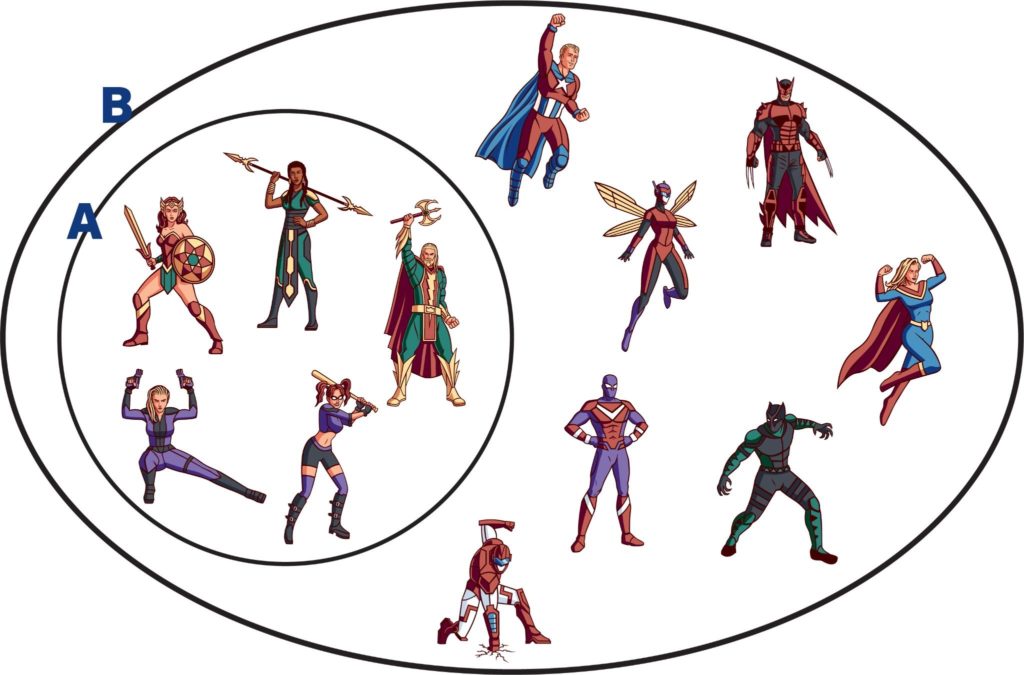
However, my guess is that the mathematical idea inspired Apache Superset as the project page proclaims that:
“Apache Superset is a modern data exploration and visualization platform that is fast, lightweight, intuitive, and loaded with options that make it easy for users of all skill sets to explore and visualize their data, from simple line charts to highly detailed geospatial charts.”
Here are some interesting points I discovered about Superset:
- It is based on SQL and can connect to any SQL database that is supported by SQL Alchemy. So at least in theory, this gives good interoperability with a large number of data sources (but also excludes some common NoSQL databases, unfortunately).
- But what if you aren’t an SQL guru? It supports a zero-code visualization builder, but also a more detailed SQL Editor.
- Superset supports more than 50 built-in charts offering plenty of choices for how you visualize your data.
- The main Superset concepts are databases, data sources, charts, and dashboards.
- It’s written in Javascript and Python.
- The focus is on “BI” (Business Intelligence) rather than machine metrics (c.f. Prometheus/Grafana) or scientific data visualization (c.f. https://matplotlib.org/ – which helped produce the 1st photograph of a black hole).
- Superset started out in Airbnb, and graduated to being a top-level Apache project this year (2021), so it’s timely to be evaluating it now.
In this blog, I wanted to get Apache Superset working with PostgreSQL. Some of the challenges I expected were:
- How easy is it to deploy Apache Superset?
- Can Apache Superset be connected to PostgreSQL (specifically, a managed Instaclustr PostgreSQL service, I had access to a preview service)?
- Is it possible to chart JSONB column data types in Apache Superset?
- Does Apache Superset have appropriate chart types to display the basic NOAA tidal data and also map the locations?
2. Deploying Apache Superset
So far in the pipeline series I’ve been used to the ease of spinning up managed services on the Instaclustr platform (e.g. Elasticsearch and Kibana). However, we currently don’t have Superset on our platform, so I was going to have to install and run it on my laptop (a Mac). I’m also used to the ease of deploying Java-based applications (get a jar, run jar). However, Superset is written in Python, which I have no prior experience with. I, therefore, tried two approaches to deploying it.
Approach 1
I initially tried to install Superset from scratch using “pip install apache-superset”. However, this failed with too many errors.
Approach 2
My second approach used Docker, which eventually (it was very slow to build) worked. I just used the built-in Mac Docker environment which worked fine—but don’t forget to increase the available memory from the default of 2GB (which soon fails) to at least 6GB. It’s also very resource-hungry while running, using 50% of the available CPU.
Superset runs in a browser at https://localhost:8088
Don’t forget to change the default user/password from admin/admin to something else.
So, given our initial false start, and by using Docker, it was relatively easy to deploy and run Superset.
3. Connecting Superset to PostgreSQL
In Superset, if you go into “Data->Databases” you find that there’s already a PostgreSQL database and drivers installed and running in the Docker version. It turns out that Superset uses PostgreSQL as the default metadata store (and for the examples).
But I wanted to use an external PostgreSQL database, and that was easy to configure on Superset following this documentation.
The PostgreSQL URL format to connect to a fully managed Instaclustr enterprise-grade service for PostgreSQL looks like this (with the pguser, pgpassword and pgip address obtained from the Instaclustr Console):
postgresql://pguser:pgpassword@pgip:5432/postgresl
Superset has the concepts of databases and datasets. After connecting to the Instaclustr managed PostgreSQL database and testing the connection you “Add” it, and then a new database will appear. After configuring a database you can add a dataset, by selecting a database, schema, and table.
So, the second challenge was also easy, and we are now connected to the external PostgreSQL database.
Instaclustr PostgreSQL Support provides a team of experts on call 24×7.
4. Apache Superset Visualization Types
Clicking on a new dataset takes you to the Chart Builder, which allows you to select the visualization type, select the time (x-axis) column (including time grain and range), and modify the query. By default, this is the “Explore” view which is the zero-code chart builder. There’s also the SQL Lab option which allows you to view and modify the SQL query.
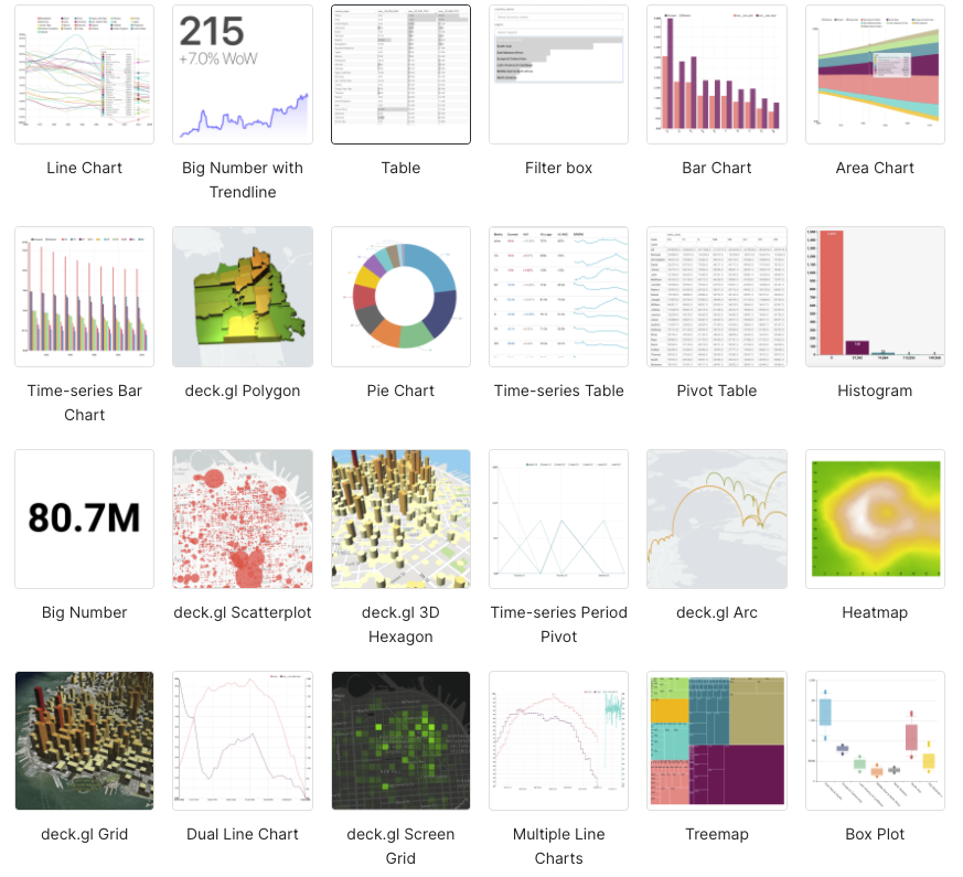
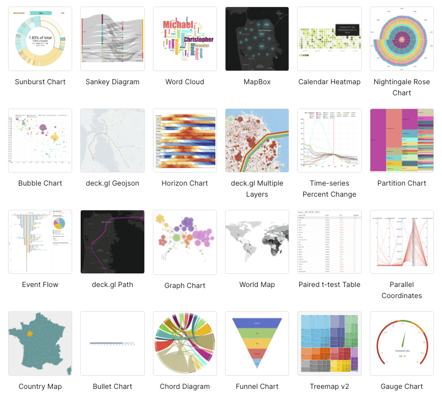
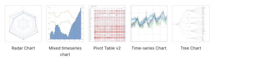
Here are the available visualization types available (which I noticed includes my favorite graph type, the Sankey diagram, which is great for systems performance analysis; Chord diagrams are also cool):
6. Charting PostgreSQL Column Data With Apache Superset
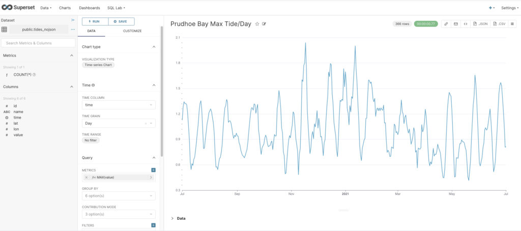
Next, I wanted to check that I could actually get data out of PostgreSQL and chart it, so I cheated (a bit) and uploaded a year’s worth of NOAA tidal data for one location using the CSV option (“Data->Upload a CSV”), which creates a table with columns in PostgreSQL, and a new corresponding dataset in Superset. From the new dataset, I created a Time-series Chart, with time as the x-axis, Day as the Time Grain, and MAX(value) as the metric. This gives the following graph showing the maximum tide height per day, so that ticks another box.
7. Charting PostgreSQL JSONB Data With Apache Superset
The real challenge was to chart the NOAA data that was streaming into my PostgreSQL database as a result of the previous blog, and which was being stored as a JSONB data type.
I created a dataset for the NOAA JSON table and tried creating a chart. Unfortunately, the automatic query builder interface didn’t have any success interpreting the JSONB data type, it just thought it was a String. So after some Googling, I found a workaround involving “virtual” datasets (JSON or Virtual datasets don’t seem to feature in the Apache documentation, unfortunately).
However, if you look at “Data->Datasets” you’ll notice that each dataset has a Type, either Physical or Virtual. Datasets are Physical by default, but you can create Virtual datasets in the SQL Lab Editor. Basically, this allows you to write your own SQL resulting in a new “virtual” table/dataset. What I needed to do was to create a SQL query that reads from the NOAA JSONB data type table and creates a new table with the columns that I need for charting, including (initially at least) the station name, time, and value.
Here’s an example of the JSON NOAA data structure:
{"metadata": {
   "id":"8724580",
   "name":"Key West",
   "lat":"24.5508”,
   "lon":"-81.8081"},
"data":[{
   "t":"2020-09-24 04:18",
   "v":"0.597",
      "s":"0.005", "f":"1,0,0,0", "q":"p"}]}
Again, after further googling and reading my blog on PostgreSQL JSON, and testing it out in the SQL Editor (you can see the results), I came up with the following SQL that did the trick:
SELECT
cast(d.item_object->>'t' as timestamp) AS __timestamp, json_object->'metadata'->'name' AS name, AVG(cast(d.item_object->>'v' as FLOAT)) AS v
FROM
tides_jsonb,jsonb_array_elements(json_object->'data')
with ordinality d(item_object, position)
where d.position=1
GROUP BY name, __timestamp;
Compared with the previous approach using Elasticsearch, this SQL achieves something similar to the custom mapping I used which overrides the default data type mappings. The difference is that using PostgreSQL you have to manually extract the correct JSON elements for each desired output column (using the “->>” and “->” operators), and cast them to the desired types. The functions “jsonb_array_elements” and “ordinality” are required to extract the first (and only) element from the ‘data’ array (into d), which is used to get the ‘v’ and ‘t’ fields.
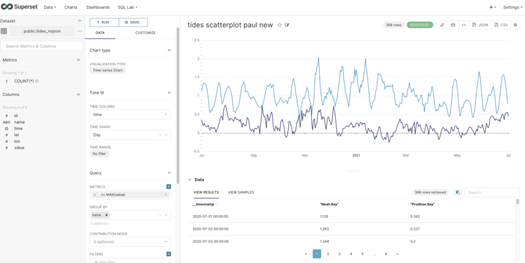
Once you’ve got this working, you click on the Explore button and “Save or Overwrite Dataset” to save the query as a virtual dataset. The new dataset (with Type Virtual in the Datasets view) is now visible, and you can create a Time-series Chart for it just as we did with the sample (CSV) column table. To display multiple graphs on one chart you also have to Group by name. The (automatically generated) SQL is pretty complex, but I noticed that it’s just nesting the above virtual query in a “FROM” clause to get the virtual dataset and graph it.
Here’s the chart with data from 2 stations:
So far, so good, now let’s tackle the mapping task.
8. Mapping PostgreSQL JSONB Data
The final task I had set myself was to attempt to replicate displaying station locations on a map, which I’d previously succeeded in doing with Elasticsearch and Kibana.
The prerequisite is to add the lat/lon JSON elements to a virtual dataset as follows:
SELECT
cast(d.item_object->>'t' as timestamp) AS __timestamp, json_object->'metadata'->'name' AS name,
cast(json_object->'metadata'->>'lat' as FLOAT) AS lat,
cast(json_object->'metadata'->>'lon' as FLOAT) AS lon,
AVG(cast(d.item_object->>'v' as FLOAT)) AS v
FROM
tides_jsonb,jsonb_array_elements(json_object->'data')
with ordinality d(item_object, position)
where d.position=1
GROUP BY name, __timestamp, lat, lon
Unlike Elasticsearch/Kibana which needed a mapping to a special geospatial data type (geo_point) to work, Superset is happy with a FLOAT type.
The next step is to find a map visualization type. Typing “map” into the visualization type search box gives these results:
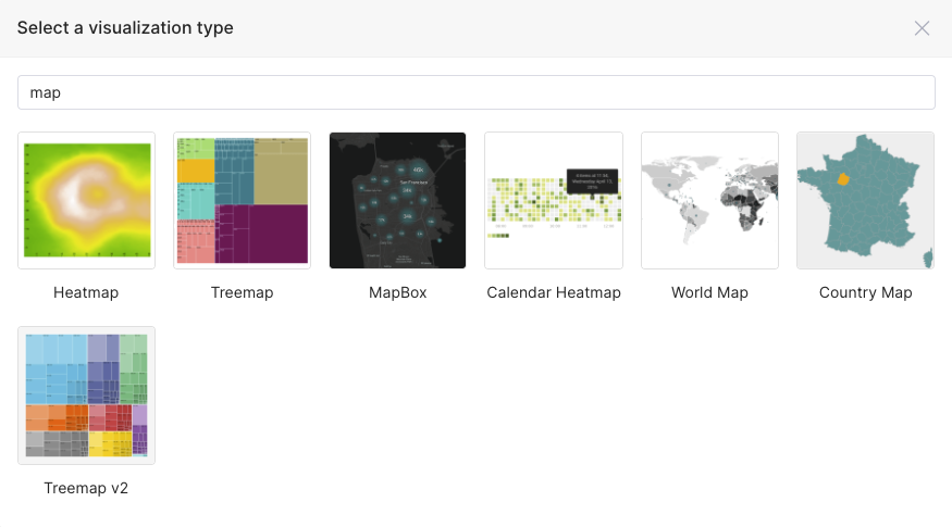
As you can see, only a few of these are actual location-based maps, and they turned out to be mainly maps for country data. I also searched for “geo” and found one map called “deck.gl Geojson”, which looked more hopeful, and searching for “deck” I found a bunch of potential candidates:
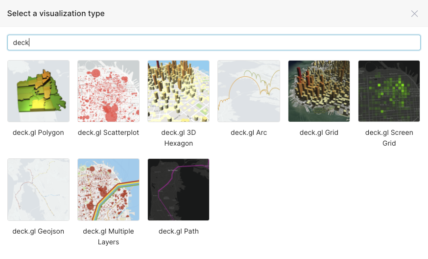
I found out that deck.gl is a framework for detailed geospatial charts so these looked promising. However, after trying a few I discovered that they didn’t have any base maps displayed. After some frantic googling, I also discovered that you need a “Mapbox” token to get them to work. You can get a free one from here. To apply the Mapbox token you have to stop the Superset Docker, go to the Superset/Docker folder, edit the non-dev config file (.env-non-dev) and add a line “MAPBOX_API_KEY = “magic number”, save it, and start superset docker again—and then the base maps will appear.
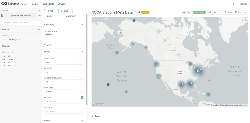
The final problem was selecting an appropriate chart type. This turned out to be trickier than I thought, as many of them have specific use cases (e.g. some automatically aggregate or cluster points). For example, the MapBox visualization successfully shows the location of the NOAA tidal stations, but at the zoomed-out level, it aggregates them and displays a count. Note that for map charts, you have to select the Longitude and Latitude columns; but watch out as this is the reverse order to the normal lat/lon order convention.
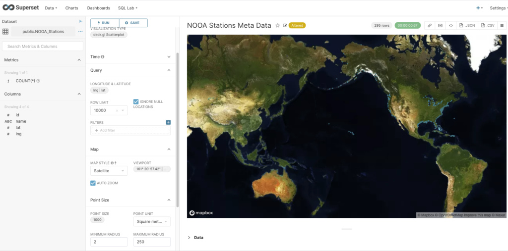
Finally the deck.gl Scatterplot visualization type (with satellite map style) succeeded in showing the location of each station (small blue dots around coastline).
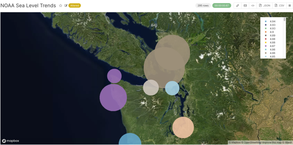
But what I really wanted to do was show a tidal value for each station location as I’d done with Kibana previously. Luckily I worked out that you can also change the size and color of the points as well. I uploaded the NOAA sea level trends (mm/year), configured point size to be based on the value with a multiplier of 10 to make them bigger, and selected Point Color->Adaptative formatting, which changes the point color based on the point size metric (unfortunately the colour gradient isn’t meaningful). Zooming in on the map you can see what this looks like in more detail, and you can easily see which tidal stations have bigger sea level trends (maybe best not to buy coastal properties there!)
9. Conclusions
How does the PostgreSQL+Superset approach compare with the previous Elasticsearch+Kibana approach?
The main difference I noticed in using them was that in Elasticsearch the JSON processing is performed at indexing time with custom mappings, whereas for Superset the transformation is done at a query-time using SQL and JSONB operators to create a virtual dataset.
In terms of interoperability, Kibana is limited to use with Elasticsearch, and Superset can be used with any SQL database (and possibly with Elasticsearch, although I haven’t tried this yet). Superset has more chart types than Kibana, although Kibana has multiple plugins (which may not be open source and/or work with Open Distro/OpenSearch).
There may also be scalability differences between the two approaches. For example, I encountered a few scalability “speed-humps” with Elasticsearch, so a performance comparison may be interesting in the future.
Get in touch to discuss a solution for your database.
Follow the Pipeline Series
- Part 1: Building a Real-Time Tide Data Processing Pipeline: Using Apache Kafka, Kafka Connect, Elasticsearch, and Kibana
- Part 2: Building a Real-Time Tide Data Processing Pipeline: Using Apache Kafka, Kafka Connect, Elasticsearch, and Kibana
- Part 3: Getting to Know Apache Camel Kafka Connectors
- Part 4: Monitoring Kafka Connect Pipeline Metrics with Prometheus
- Part 5: Scaling Kafka Connect Streaming Data Processing
- Part 6: Streaming JSON Data Into PostgreSQL Using Open Source Kafka Sink Connectors
- Part 7: Using Apache Superset to Visualize PostgreSQL JSON Data