In Part 4 of this blog series, we started exploring Kafka Connector task scalability by configuring a new scalable load generator for our real-time streaming data pipeline, discovering relevant metrics, and configuring Prometheus and Grafana monitoring. We are now ready to increase the load and scale the number of Kafka Connector tasks and demonstrate the scalability of the stream data pipeline end-to-end. 

1. Scaling Kafka Connector Tasks

Kafka scalability is determined largely by the number of partitions and client consumers you have (noting that partitions must be >= consumers). For Kafka sink connectors, the number of connector tasks corresponds to the number of Kafka consumers running in a single consumer group. 

But watch out! You can easily start instances of the same connector in different consumer groups (simply by changing the connector name in the config file and restarting). This may be what you want (for example, to send data to multiple Elasticsearch clusters), but it may also just be an accident (when debugging and testing). This will result in increased load and duplicate records sent to the sink system—and can be quite hard to detect.

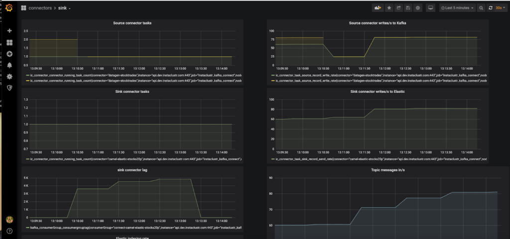
Having the end-to-end Prometheus pipeline metrics in a single Grafana dashboard made it very easy to see what was going on in terms of throughput and lag, all the way from the source connector input rate, the topic rate, the sink connector rate, and the Elasticsearch index rate, aided by the sink connector consumer group lag. 

To ensure steady-state throughput, the input and output rates need to be comparable. The lag also needs to be as close to zero as possible, and definitely not increasing. There’s no way to measure end-to-end latency with the available Kafka and Elasticsearch metrics that I have been able to find so far, but latency can be estimated using Little’s Law: the average number of users in a system (U), is the average throughput (TP), multiplied by the average time spent in the system (RT):

U = RT x TP

This is one of the few times when an average is the correct statistic to use for system performance!

Rearranging for RT (time), we get:

RT = U/TP

Surprisingly (well, I’m always surprised), Little’s Law works for “anything”, even desert Camel races! 

For example, if U (the number of Camels in a race) = 20, and TP (the average throughput, or the number of camels crossing the finishing line per second) = 0.333 (1 camel every 3s), then the average time for camels to complete the race is 20/0.333 = 60s. 

For our pipeline problem, U = lag, and TP is the rate.  For example, the latency (RT) for a lag of 2 and rate of 40 is 50ms, and for a lag of 200 and a rate of 200 is 1s, probably about the maximum tolerable for a close to real-time use case (e.g. stock tickers). But it’s only an average, so some records may take a lot longer to arrive. If the lag increases to say 10,000 then you obviously have a problem, as the RT is heading to minutes not seconds.

This metric could be computed and displayed by Prometheus/Grafana, but you’d need some PromQL magic to do it as Prometheus only allows you to combine metrics with operators if they have the “same dimensional labels” (lag and rate have different dimensions). This would do the trick. :

The other observation is that once the lag starts to increase it can take a long time for it to drop back again, even if the input rate decreases, and even if you increase the number of tasks. This is because it’s far easier to push more events into Kafka than it is to get them out and send them to Elasticsearch—as we’ll now see.

Now I wanted to see how easy it is to scale the system with increasing input rates using the Kafka connect source data generator. To scale the Kafka connector side you have to increase the number of tasks, ensuring that there are sufficient partitions.

In theory, you can set the number of partitions to a large number initially, but in practice, this is a bad idea. Kafka throughput is optimal when the number of partitions is between the number of threads in the cluster and 100. Over 100 partitions and the throughput drops significantly. See this blog for more details. 

My methodology was straightforward. I set the number of partitions to 20 (which is < 100, and > number of vCPUs), started with a single sink connector task, and increased the input load until the sink connector lag increased and the sink connector output rates couldn’t keep up. 

I determined that the maximum sustainable throughput for a single Camel Elasticsearch sink connector task is around 70 per second. This implies that Elasticsearch indexing is substantially slower than Kafka reads.  Using Little’s Law again, the connector task latency = 1/70 = 14ms. 

Here’s the corresponding screenshot of the Grafana dashboard (excluding the elastic index rate metric which didn’t fit on the screen). The bottom-left graph is the lag, and shows that the sink connector got behind for a while, increasing the lag, but then caught up again, and the lag dropped to close to zero (which reduces the latency to close to zero).

2. Speed Humps: Scaling Kafka Connector Tasks

“Would you like one hump or two?” (That’s a Camel joke).  While scaling I encountered two speed humps as follows.

First Speed Hump (Dromedary Camel)

Adding extra tasks should increase the total throughput roughly linearly. I tried 2 tasks and achieved 140 index operations a second as expected. But with 3 tasks I ran into a surprise! Three tasks actually only achieved the same throughput as two, which was “unexpected”. However, this was an occasion where graphing the per task metrics (not just the sum) was useful. It was apparent from the “Sink connector writes to Elasticsearch” graph that 1 of the 3 tasks had zero throughputs. So what’s going on?  

I mentioned in Part 4 that initially I didn’t configure the datagen configuration file with an explicit “keyfield”. It turns out that by default datagen uses the first field in the JSON record as the Kafka topic key, which was “side” in this example. But “side” only has two distinct values, so you can’t sensibly scale the number of partitions beyond two.

Fundamentally, if you don’t have sufficient values for a key, some of the partitions will be empty and therefore some consumers will be starved of records to process.  For more information on Kafka key and partition scaling see the “Key Parking Problem” section of this blog.  My rule of thumb is to have more than ten (twenty is good) times more key values than partitions.

To solve this problem I explicitly set the keyfield to a field that had lots of values, price, by adding the following line to the Kafka source connector configuration:

After restarting the datagen connector, the 3 sink tasks were all processing similar numbers of records and in total achieved the expected 210 indexing operations per second throughput.

Second Speed Hump (Bactrian Camel)

Next, I decided to check the Instaclustr console for each of the clusters to ensure that the hardware resources were not hitting any limits. The CPU utilization on the Kafka and Kafka connect clusters was minimal (even though they were only small test clusters—3 node x 2 vCPUs per node).

But, with Kafka connect there are always (mostly, datagen doesn’t involve a sink system) multiple systems (source and sink systems, plus Kafka). So, how well was the Elasticsearch sink system working?

The one odd thing I noticed was that the CPU utilization on the Elasticsearch cluster was also almost entirely on one node, and getting close to the maximum, which was surprising. Clarifying the expected cluster behavior with our Elasticsearch experts, we discovered that that the default shards per index changed from 5 shards to 1 shard per index in Elasticsearch 7.0. Instaclustr currently runs Open Distro for Elasticsearch version 1.8.0, which corresponds to Elasticsearch 7.7.0, so this was obviously the issue.

Given that a shard is a single threaded Lucene instance, this may not be a good default for Elasticsearch clusters for higher indexing rates. A single shard is not scalable, either in terms of utilizing multiple CPU cores or multiple cluster nodes. Determining the optimal number of shards isn’t trivial, and depends on multiple factors including cluster size and topology, read and write workloads, number of indices, and available memory.

The default number of shards for new indices can be changed as follows. For example, to 3 shards, so that the shards which will be distributed across more nodes in the Elasticsearch cluster resulting in more even distribution and higher throughput:

Given that our Prometheus configuration file has been set up with metrics for only 5 Elasticsearch sink tasks, this seemed like a sensible (but arbitrary) target number of tasks to aim for. Increasing the Elasticsearch tasks, with 1 Elasticsearch index shard still, proves that this is probably the bottleneck, with a maximum of 270 index operations a second, not much more than the 3 task throughput.

Creating a new index (as you can’t easily increase the number of shards on an existing index) with 3 shards and 2 replicas, and rerunning the experiment with 5 tasks, gives the expected results, 350 index operations per second (350 = 70 x 5).

3. Conclusions

With Kafka Connect there’s no theoretical upper limit to the streaming data scalability that can be achieved, and Kafka clusters can easily cope with millions of events per second flowing through them. However, for this experiment, I stopped scaling with 5 connector tasks, as I hadn’t really provisioned the clusters for more serious scaling or benchmarking.

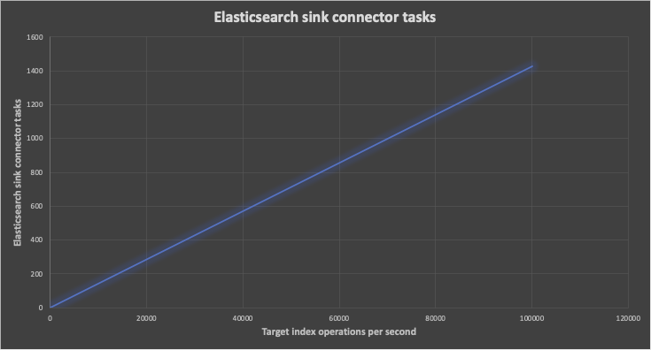
The below graph shows the predicted minimum number of Elasticsearch sink connector tasks (y-axis) required to achieve increasing target index operations per second (x-axis). For example, for 10,000 index operations per second, at least 142 tasks are predicted—probably more due to the negative impact of increasing partitions on Kafka cluster throughput:

So what can we conclude about Kafka connect pipeline scalability?

Throughput certainly increases with increasing tasks, but you also have to ensure that the number of distinct key values is high enough, that the number of partitions is sufficient (but not too many), and also keep an eye of the cluster hardware resources, particularly the target sink system, as it’s easy to have a high throughput pipeline on the Kafka side, but overload slower target sink systems.

This is one of the catches of using Kafka connect, as there are always two (three really) systems involved—the source, Kafka, and sink sides—so monitoring and expertise is required to ensure a smooth flowing pipeline across multiple systems.

Of course, an important use case of Kafka is to act as a buffer, as in general, it’s not always feasible to ensure comparable capacities for all systems involved in a pipeline or for them to be perfectly elastic—increasing resource takes time (and money), and for some applications being able to buffer the events in Kafka while sink systems eventually catch up may be the prime benefit of having Kafka connect in the pipeline (My Anomalia Machina blog series and ApacheCon 2019 talk cover Kafka as a buffer).

The number of Kafka connector tasks may also be higher than expected if you have a mismatch between systems (i.e. one is a lot slower than the other), as this introduces latency in the connector which requires increased concurrency to increase throughput to the target rate. There may be some “tricks”—for example, Elasticsearch supports a Bulk indexing API (but this would require support from the connector to use it, which is what the Aggregator is for).

Finally, if you care about end-to-end latency, don’t let the input rate exceed the pipeline processing capacity, as the lag will rapidly increase pushing out the total delivery latency. Even with sufficient attention to monitoring, it’s tricky to prevent this, as I noticed that restarting the Kafka sink connectors with more tasks actually results in a drop in throughput for 10s of seconds (due to consumer group rebalancing), momentarily increasing the lag.

Moreover, event based systems typically have open (vs. closed) workloads and don’t receive input events at a strictly constant/average rate, so the arrival distribution is often Poisson (or worse). This means you can get a lot more than the average number of arrivals in any time period, so you need more processing capacity (headroom) than the average rate to prevent backlogs.

We, therefore, recommend that you benchmark and monitor your Kafka connect applications to determine adequate cluster sizes (number of nodes, node types, etc.) and configuration (number of Kafka connector tasks, topic partitions, Elasticsearch shards, and replicas, etc.) for your particular use case, workload arrival rates and distributions, and SLAs.

Thereby achieving “Humphrey” scaling! (“What do you call a Camel with no humps?”…)

Surprisingly you can also call a camel with no humps “Llama”, as Llamas (along with Alpacas, Guanacos, and Vicunas) are members of the camel family with no humps!

(Source: Shutterstock)

That’s the end of our “Building a Real-Time Tide Data Processing Pipeline: Using Apache Kafka, Kafka Connect, Camel Kafka Connector, Elasticsearch, and Kibana” series. We started out at the Ocean (with tidal data), trekked through the desert with Apache Camel Kafka Connector, and ended up in the mountains with llamas (thereby inverting the normal source-to-sink—mountains to oceans—journey of water, but water is a cycle so water just keeps on moving around). You can look in the individual blogs for the example configuration files we used during the series, but we’ve also put them together in Github.

Follow the Pipeline Series

• Part 1: Building a Real-Time Tide Data Processing Pipeline: Using Apache Kafka, Kafka Connect, Elasticsearch, and Kibana
• Part 2: Building a Real-Time Tide Data Processing Pipeline: Using Apache Kafka, Kafka Connect, Elasticsearch, and Kibana
• Part 3: Getting to Know Apache Camel Kafka Connectors
• Part 4: Monitoring Kafka Connect Pipeline Metrics with Prometheus
• Part 5: Scaling Kafka Connect Streaming Data Processing
• Part 6: Streaming JSON Data Into PostgreSQL Using Open Source Kafka Sink Connectors
• Part 7: Using Apache Superset to Visualize PostgreSQL JSON Data
• Part 8: Kafka Connect Elasticsearch vs. PostgreSQL Pipelines: Initial Performance Results
• Part 9: Kafka Connect and Elasticsearch vs. PostgreSQL Pipelines: Final Performance Results
• Part 10: Comparison of Apache Kafka Connect, Plus Elasticsearch/Kibana vs. PostgreSQL/Apache Superset Pipelines