This is the third (and final) part of my blog-series on creating a demonstration Cassandra cluster, connecting, and communicating. We landed on the moon and made Second Contact with the Monolith (CQL shell) in our last blog, but what can we do to understand the Monolith better? Let’s explore Cassandra Java client program.
Java Client Driver
Apart from the CQL shell, another way of connecting to Cassandra is via a programming language driver. I’ll use Java. Instaclustr has a good introduction to Cassandra and Drivers, including best practices for configurations. We recommend the DataStax driver for Java which is available under the Apache license as a binary tarball. Unpack it and include all the jar files in your Java libraries build path (I use Eclipse so I just had to import them). The driver documentation is here, and this is a good summary.
Connection
From the Instaclustr console, under your trial cluster, Connection Info tab, at the bottom are code samples for connecting to the trial cluster with pre-populated data.
Cassandra Java Client example
This is a simplistic code example of connecting to the trial Cassandra cluster, creating a time series data table, filling it with realistic looking data, querying it and saving the results into a csv file for graphing (Code below). To customise the code for your cluster, change the public IP addresses, and provide the data centre name and user/password details (it’s safest to use a non-super user). The Cluster.builder() call uses a fluent API to configure the client with the IP addresses, load balancing policy, port number and user/password information. I’ve obviously been under a rock for a while as I havn’t come across fluent programming before. It’s all about the cascading of method invocations, and they are supported in Java 8 by Lambda functions (and used in Java Streams). This is a very simple configuration which I’ll revisit in the future with the Instaclustr recommended settings for production clusters.
The program then builds, gets meta data and prints out the host and cluster information, and then creates a session by connecting. You have the option of dropping the test table if it already exists or adding data to the existing table.
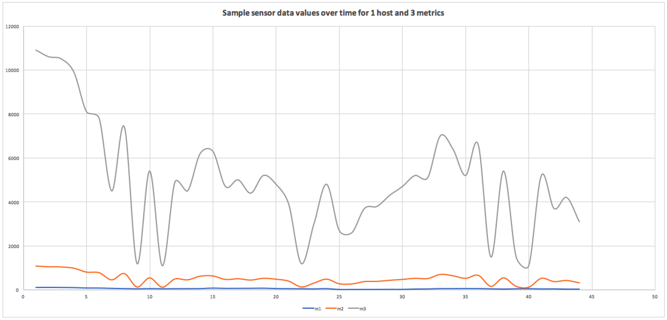
Next, we fill the table with some realistic time series sensor data. You can change how many host names (100 by default) are used, and how many timestamps are generated. For each time 3 metrics and values will be inserted. There are several types of statements in the Java clients including simple and prepared statements. In theory prepared statements are faster so there’s an option to use either in the code. In practice it seems that prepared statements may not improve response time significantly but may be designed to improve throughput. Realistic looking data is generated by a simple random walk.
The code illustrates some possible queries (SELECTs), including a simple aggregate function (max) and retrieving all the values for one host/metric combination, finding all host/metric permutations (to assist with subsequent queries as we made the primary key a compound key of host and metric so both are needed to select on), and finally retrieving the whole table and reporting the number of rows and total bytes returned.
What does the data look like?
The simplest possible way of taking a better look at the data was to use the cqlsh again and run this command to produce a CSV file:
COPY hals.sensordata TO ‘../test1.csv’ WITH header=true;
You can then read the csv file into excel (or similar) and graph (for example) all the metric values over time for a selected host:
|
1 2 3 4 5 6 7 8 9 10 11 12 13 14 15 16 17 18 19 20 21 22 23 24 25 26 27 28 29 30 31 32 33 34 35 36 37 38 39 40 41 42 43 44 45 46 47 48 49 50 51 52 53 54 55 56 57 58 59 60 61 62 63 64 65 66 67 68 69 70 71 72 73 74 75 76 77 78 79 80 81 82 83 84 85 86 87 88 89 90 91 92 93 94 95 96 97 98 99 100 101 102 103 104 105 106 107 108 109 110 111 112 113 114 115 116 117 118 119 120 121 122 123 124 125 126 127 128 129 130 131 132 133 134 135 136 137 138 139 140 141 142 143 144 145 146 147 148 149 150 151 152 153 154 155 156 157 158 159 160 161 162 163 164 165 166 |
package test1; import java.util.Date; import com.datastax.driver.core.*; import com.datastax.driver.core.policies.DCAwareRoundRobinPolicy; /* * Simple Java client test to connect to trial cluster, create a time series data table, fill it, query it, and save it as csv for graphing. */ public class CassTest1 { // the 3 node trial Cassandra test cluster Public IPs. These are dummy values. static String n1PubIP = "01.23.45.678"; static String n2PubIP = "01.234.56.78"; static String n3PubIP = "01.23.456.78"; static String dcName = "hal_sydney"; // this is the DC name you used when created static String user = "user"; static String password = "password"; public static void main(String[] args) { long t1 = 0; // time each CQL operation, t1 is start time t2 is end time, time is t2-t1 long t2 = 0; long time = 0; Cluster.Builder clusterBuilder = Cluster.builder() .addContactPoints( n1PubIP, n2PubIP, n3PubIP // provide all 3 public IPs ) .withLoadBalancingPolicy(DCAwareRoundRobinPolicy.builder().withLocalDc(dcName).build()) // your local data centre .withPort(9042) .withAuthProvider(new PlainTextAuthProvider(user, password)); Cluster cluster = null; try { cluster = clusterBuilder.build(); Metadata metadata = cluster.getMetadata(); System.out.printf("Connected to cluster: %s\n", metadata.getClusterName()); for (Host host: metadata.getAllHosts()) { System.out.printf("Datacenter: %s; Host: %s; Rack: %s\n", host.getDatacenter(), host.getAddress(), host.getRack()); } Session session = cluster.connect(); ResultSet rs; boolean createTable = true; if (createTable) { rs = session.execute("CREATE KEYSPACE IF NOT EXISTS hals WITH replication = {'class': 'SimpleStrategy', 'replication_factor' : 3}"); rs = session.execute("DROP TABLE IF EXISTS hals.sensordata"); rs = session.execute("CREATE TABLE hals.sensordata(host text, metric text, time timestamp, value double, PRIMARY KEY ((host, metric), time) ) WITH CLUSTERING ORDER BY (time ASC)"); System.out.println("Table hals.sensordata created!"); } // Fill the table with some realistic sensor data. if createTable=false we just ADD data to the table double startValue = 100; // start value for random walk double nextValue = startValue; // next value in random walk, initially startValue int numHosts = 100; // how many host names to generate int toCreate = 1000; // how many times to pick a host name and create all metrics for it boolean usePrepared = false; PreparedStatement prepared = null; // prepare a prepared statement if (usePrepared) { System.out.println("Using PREPARED statements for INSERT"); prepared = session.prepare("insert into hals.sensordata (host, metric, time, value) values (?, ?, ?, ?)"); } t1 = System.currentTimeMillis(); System.out.println("Creating data... iterations = " + toCreate); for (int r=1; r <= toCreate; r++) { long now = System.currentTimeMillis(); Date date = new Date(now); // generate a random host name String hostname = "host" + (long)Math.round((Math.random() * numHosts)); // do a random walk to produce realistic data double rand = Math.random(); if (rand < 0.5) // 50% chance that value doesn't change ; else if (rand < 0.75) // 25% chance that value increases by 1 nextValue++; else // 25% chance that value decreases by 1 nextValue--; // never go negative if (nextValue < 0) nextValue = 0; // comparison of prepared vs. non-prepared statements if (usePrepared) { session.execute(prepared.bind("'" + hostname + "'", "'m1'", date, nextValue)); session.execute(prepared.bind("'" + hostname + "'", "'m2'", date, nextValue * 10)); session.execute(prepared.bind("'" + hostname + "'", "'m3'", date, nextValue * 100)); } else { // fake three metrics (m1, m2, m3) which are somehow related. rs = session.execute("insert into hals.sensordata (host, metric, time, value) values (" + "'" + hostname + "'" + ", " + "'m1'" + ", " + now + "," + (nextValue) + ");" ); rs = session.execute("insert into hals.sensordata (host, metric, time, value) values (" + "'" + hostname + "'" + ", " + "'m2'" + ", " + now + "," + (nextValue * 10) + ");" ); rs = session.execute("insert into hals.sensordata (host, metric, time, value) values (" + "'" + hostname + "'" + ", " + "'m3'" + ", " + now + "," + (nextValue * 100) + ");" ); } } t2 = System.currentTimeMillis(); System.out.println("Created rows = " + toCreate*3 + " in time = " + (t2-t1)); // find the max value for a sample System.out.println("Getting max value for sample..."); t1 = System.currentTimeMillis(); rs = session.execute("select max(value) from hals.sensordata where host='host1' and metric='m1'"); t2 = System.currentTimeMillis(); time = t2-t1; Row row = rs.one(); System.out.println("Max value = " + row.toString() + " in time = " + time); // get all the values for a sample System.out.println("Getting all rows for sample..."); t1 = System.currentTimeMillis(); rs = session.execute("select * from hals.sensordata where host='host1' and metric='m1'"); for (Row rowN : rs) { System.out.println(rowN.toString()); } t2 = System.currentTimeMillis(); time = t2-t1; System.out.println("time = " + time); // get all host/metric permutations System.out.println("Getting all host/metric permutations"); t1 = System.currentTimeMillis(); rs = session.execute("select distinct host, metric from hals.sensordata"); for (Row rowN : rs) { System.out.println(rowN.toString()); } t2 = System.currentTimeMillis(); time = t2-t1; System.out.println("time = " + time); // Note that SELECT * will return all results without limit (even though the driver might use multiple queries in the background). // To handle large result sets, you use a LIMIT clause in your CQL query, or use one of the techniques described in the paging documentation. System.out.println("Select ALL..."); t1 = System.currentTimeMillis(); rs = session.execute("select * from hals.sensordata"); System.out.println("Got rows (without fetching) = " + rs.getAvailableWithoutFetching()); int i = 0; long numBytes = 0; // example use of the data: count rows and total bytes returned. for (Row rowN : rs) { i++; numBytes += rowN.toString().length(); } t2 = System.currentTimeMillis(); time = t2-t1; System.out.println("Returned rows = " + i + ", total bytes = " + numBytes + ", in time = " + time); } finally { if (cluster != null) cluster.close(); } } } |
Next blog: A voyage to Jupiter: Third Contact with a Monolith—exploring real Instametrics data.
Don’t have a trial cluster?