In Part 1 of this series, we had a look at Kafka concurrency and throughput work, recapped some earlier approaches I used to improve Kafka performance, and introduced the Kafka Parallel Consumer and supported ordering options (Partition, Key, and Unordered). In this second part we continue our investigations with some example code, a trace of a “slow consumer” example, how to achieve 1 million TPS in theory, some experimental results, what else do we know about the Kafka Parallel Consumer, and finally, if you should use it in production. 

This is a closeup of the “mystery machine” from Part 1 (a Jacquard programmable loom).

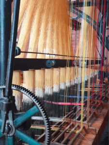
Jacquard loom from the foyer of the Deutsches Technikmuseum, Berlin

(Source: Paul Brebner)

1. Example Parallel Consumer Code

Here’s a simple example of the Parallel Consumer. The consumer options can be found in this file. There are some things to watch out for, however: 

1. Auto Commit must be turned off, as the Parallel Consumer handles commits itself. So, in the consumer configuration, set enable.auto.commit=false. 
2. Decide on the ordering mode. Options are ProcessingOrder.PARTITION, ProcessingOrder.KEY and ProcessingOrder.UNORDERED. These are set in the ParallelConsumerOptions builder, e.g., ordering(ProcessingOrder.KEY). 
3. Choose your concurrency level—this is the maximum number of threads used for the record processing thread pool, also set in the builder, this can be anything from 1 to lots, e.g., maxConcurrency(100). Set this based on knowledge of client resources and Partition or Key space sizes. 
4. Choose what type of consumer to use—I used the ParallelStreamProcessor. 
5. Provide a function containing the record processing logic. This example just sleeps for 1s and prints out the end-to-end latency, so it’s easy to see what’s going on. 
6. Only poll once (unlike the default consumer).

Here’s the code: 

2. Some “Slow Consumer” Latency Examples

Do you remember this shipping incident from 2021? The container ship, the “Ever Given” (owned by the company Evergreen, hence the name on the ship) was stuck in the Suez Canal for 6 days. Some sections of the Suez Canal are “one lane” only—so a blockage can result in very long delays for other ships. Over 300 ships were queued up waiting to get through, and it took days to clear the backlog once the canal was unblocked. 

(Source: Shutterstock)

So, let’s take a look at the impact of 1 vs. many lanes (concurrency) and unexpected slow records, using a trace of some simple experiments with the Kafka Parallel Consumer. For each experiment, we’ll send 10 records to a topic, have a single consumer subscribed to the topic, and print out the total end-to-end latency, including record processing time, for each record, and the partition, key, and value (“hello 0” to “hello 9”, sent in order).

For the first experiment, there is 1 partition, 1 consumer, and 1 thread, 1 key per record, and 1 second processing time per record (we set this high so that it’s easy to see what’s going on), and ordering by Partition:

Parallel processing record time latency= 1035, partition=0, key=0, value=hello 0
Parallel processing record time latency= 2014, partition=0, key=1, value=hello 1
Parallel processing record time latency= 3013, partition=0, key=2, value=hello 2
Parallel processing record time latency= 4015, partition=0, key=3, value=hello 3
Parallel processing record time latency= 5014, partition=0, key=4, value=hello 4
Parallel processing record time latency= 6012, partition=0, key=5, value=hello 5
Parallel processing record time latency= 7013, partition=0, key=6, value=hello 6
Parallel processing record time latency= 8012, partition=0, key=7, value=hello 7
Parallel processing record time latency= 9010, partition=0, key=8, value=hello 8
Parallel processing record time latency= 10013, partition=0, key=9, value=hello 9

The end-to-end latency increases by approximately 1s per record, as the records are processed sequentially in order as there’s only a single partition. The latency for each record increases as they have to wait for all the preceding records obtained by the consumer poll to be processed. the biggest latency is just over 10s (10 x 1s). 

What can we do to improve performance? Let’s repeat this experiment with 2 partitions and increase the consumer concurrency to 10: 

Parallel processing record time latency= 1036, partition=0, key=0, value=hello 0
Parallel processing record time latency= 1011, partition=1, key=1, value=hello 1
Parallel processing record time latency= 1961, partition=0, key=2, value=hello 2
Parallel processing record time latency= 1964, partition=1, key=3, value=hello 3
Parallel processing record time latency= 2902, partition=0, key=5, value=hello 5
Parallel processing record time latency= 2945, partition=1, key=4, value=hello 4
Parallel processing record time latency= 3886, partition=0, key=6, value=hello 6
Parallel processing record time latency= 3883, partition=1, key=7, value=hello 7
Parallel processing record time latency= 4869, partition=1, key=8, value=hello 8
Parallel processing record time latency= 5857, partition=1, key=9, value=hello 9

The first thing to notice is that the records are not being processed strictly in the same order that they were sent now, as there are a couple out of order (“hello 5” and “hello 4”). This is because we have a concurrency of 2 for the consumer now, with the records for each of the 2 partitions being processed in sequence. The messages are in order by partition (for partition 0: messages 0, 2, 5, 6; for partition 1: messages 1, 3, 4, 7, 8, 9, and because the concurrency is 2 the end-to-end latency has improved, with the biggest latency now reduced from 10s to 5.8s. Note that for such a simple example with only 10 messages we didn’t get a perfect improvement as there were 4 records in partition 0, and 6 in the other, so records were processed faster for partition 0 c.f. Partition 1.  

What happens if we now increase the partition count to 10 (consumer concurrency is still 10)? Do we get a maximum of 1s latency?

Parallel processing record time latency= 1034, partition=6, key=0, value=hello 0
Parallel processing record time latency= 1012, partition=9, key=1, value=hello 1
Parallel processing record time latency= 1009, partition=8, key=2, value=hello 2
Parallel processing record time latency= 1013, partition=3, key=3, value=hello 3
Parallel processing record time latency= 1012, partition=0, key=5, value=hello 5
Parallel processing record time latency= 1012, partition=7, key=8, value=hello 8
Parallel processing record time latency= 1877, partition=9, key=7, value=hello 7
Parallel processing record time latency= 1926, partition=8, key=6, value=hello 6
Parallel processing record time latency= 1995, partition=3, key=4, value=hello 4
Parallel processing record time latency= 2898, partition=3, key=9, value=hello 9

Apparently not. The maximum latency has reduced again to 2.8s, but this isn’t 1s. Again, we notice that with 10 records and 10 partitions, the records are not perfectly balanced over the partitions. In fact, only 6 partitions have any records, with 1 to 3 records per partition (hence the close to 3s maximum latency). The messages are being delivered in order by partition still (although they are even more out of sending order than before). 

So, it’s apparent for this simple example at least) that ordering by Partition reduces the end-to-end latency because of the concurrent processing, but that the improvement isn’t as good as theory suggests due to limitations around the number of partitions and the uneven distribution of records across partitions. 

So, let’s try the next ordering option, by Key (and reverting to the original 1 partition but with consumer concurrency 10): 

Parallel processing record time latency= 1013, partition=0, key=1, value=hello 1
Parallel processing record time latency= 1013, partition=0, key=2, value=hello 2
Parallel processing record time latency= 1013, partition=0, key=3, value=hello 3
Parallel processing record time latency= 1011, partition=0, key=4, value=hello 4
Parallel processing record time latency= 1011, partition=0, key=5, value=hello 5
Parallel processing record time latency= 1013, partition=0, key=6, value=hello 6
Parallel processing record time latency= 1010, partition=0, key=7, value=hello 7
Parallel processing record time latency= 1011, partition=0, key=8, value=hello 8
Parallel processing record time latency= 1013, partition=0, key=9, value=hello 9

This is a big improvement as the maximum is now 1s and the records are delivered in sending order. What’s going on? Because we have 10 keys and each record has a unique key we are utilizing the full 10 consumer threads, so they are all processed at once (and therefore have a similar latency time of 1s).

Let’s now try the final ordering option, Unordered, still with consumer concurrency 10:

Parallel processing record time latency= 1032, partition=6, key=0, value=hello 0
Parallel processing record time latency= 1014, partition=9, key=1, value=hello 1
Parallel processing record time latency= 1013, partition=8, key=2, value=hello 2
Parallel processing record time latency= 1010, partition=3, key=3, value=hello 3
Parallel processing record time latency= 1013, partition=3, key=4, value=hello 4
Parallel processing record time latency= 1012, partition=0, key=5, value=hello 5
Parallel processing record time latency= 1012, partition=8, key=6, value=hello 6
Parallel processing record time latency= 1009, partition=9, key=7, value=hello 7
Parallel processing record time latency= 1012, partition=7, key=8, value=hello 8
Parallel processing record time latency= 1008, partition=3, key=9, value=hello 9

These results look identical to the previous Key ordered results. This is logical as the concurrency is the same (10), and each record is processed independently of the others. They both process records in the order of sending, but is this just a coincidence? Let’s see what happens when one of the events is significantly slower than the others, in this case “hello 5” (“Ever Given” would have been a more appropriate value) has a 5s processing time: 

Parallel processing record time latency= 1018, partition=9, key=1, value=hello 1
Parallel processing record time latency= 1015, partition=8, key=2, value=hello 2
Parallel processing record time latency= 1014, partition=3, key=3, value=hello 3
Parallel processing record time latency= 1011, partition=3, key=4, value=hello 4
Parallel processing record time latency= 1014, partition=8, key=6, value=hello 6
Parallel processing record time latency= 1012, partition=9, key=7, value=hello 7
Parallel processing record time latency= 1014, partition=7, key=8, value=hello 8
Parallel processing record time latency= 1011, partition=3, key=9, value=hello 9
Parallel processing record time latency= 5011, partition=0, key=5, value=hello 5

Not surprisingly, “hello 5” (bolded) is now delayed, has a latency of 5s, and arrives last and out of order. However, none of the other records are held up by this slow record so the impact is minimal. 

But what if we really want records delivered in order? Let’s revert to the Key ordering and see if we can improve things, this time with 2 distinct Keys only:

Parallel processing record time latency= 1033, partition=6, key=0, value=hello 0
Parallel processing record time latency= 1011, partition=9, key=1, value=hello 1
Parallel processing record time latency= 1961, partition=6, key=0, value=hello 2<
Parallel processing record time latency= 1967, partition=9, key=1, value=hello 3
Parallel processing record time latency= 2919, partition=6, key=0, value=hello 4
Parallel processing record time latency= 3877, partition=6, key=0, value=hello 6
Parallel processing record time latency= 4844, partition=6, key=0, value=hello 8
Parallel processing record time latency= 6921, partition=9, key=1, value=hello 5
Parallel processing record time latency= 7885, partition=9, key=1, value=hello 7
Parallel processing record time latency= 8854, partition=9, key=1, value=hello 9

The order per key is correct, i.e., Key 0 -> 0, 2, 4, 6, 8, and Key 1 -> 1, 3, 5, 7, 9 

However, the latency is longer (8.8s), as the slow “hello 5” record results in a delay to the subsequent records in Key. 

3. How to Achieve 1 million TPS?

In this section, we show the results of a simple model that uses Little’s Law (Concurrency = Response Time x Throughput) to show the impact of using the default consumer vs. the parallel consumer. The goal is to process 1 million records a second. We make several assumptions. The first is that each partition can process a maximum of 10,000 records/s, so to process 1M records/s we need a minimum of 100 partitions. Second, we assume a single consumer group is subscribed to the topic. If more than one group is subscribed, then the number of partitions needs to be increased to cope with the total throughput across all the groups. Default consumers are only single-threaded, so to process 1M records/s we also need 100 consumers. This is assuming there is zero consumer side processing time for the events (they are simply read from a topic and discarded), giving the best-case result for the default consumer shown on the left of the graph, (1) the first pair of bars for 100 partitions (blue) and 100 consumers (orange). Note that the graph has a logarithmic y-axis.  

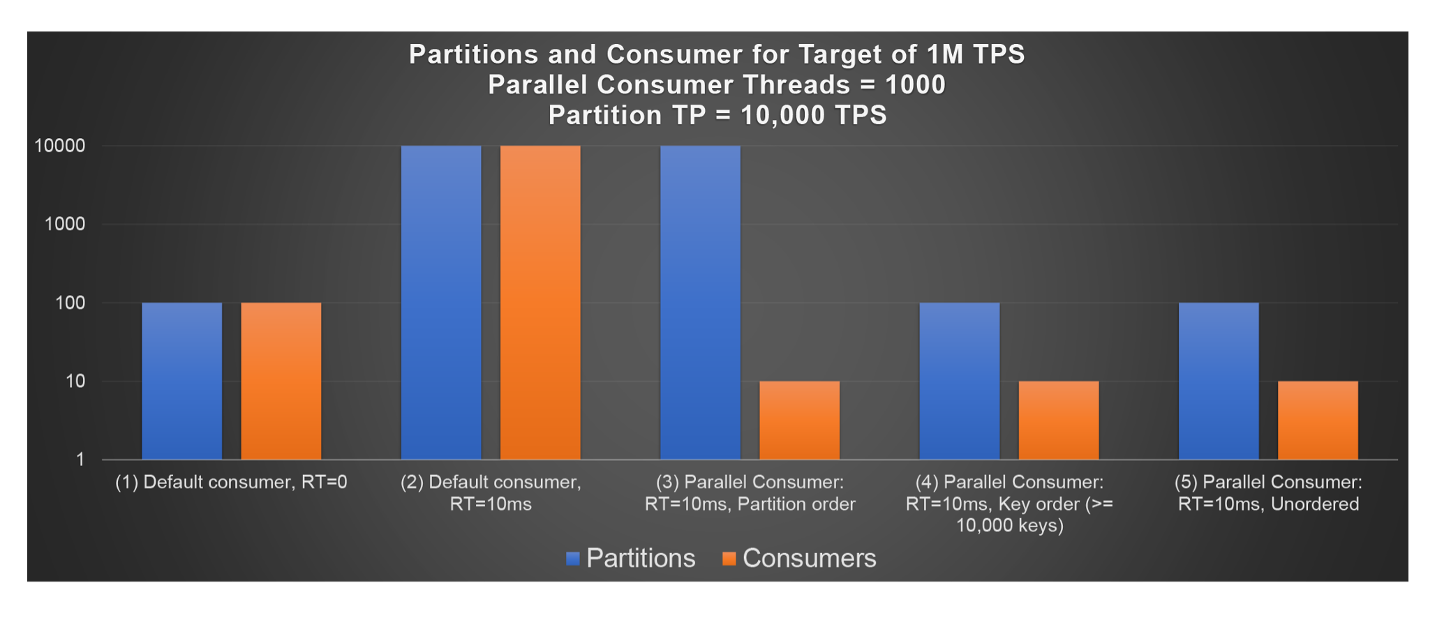
Let’s now see what happens when we increase the record processing time to 10ms. Firstly, for the default consumer, this is challenging, as Little’s Law predicts that as the response time increases, then concurrency must also increase to compensate. In fact, to process 1M records/s a second with a 10m processing time, we need a system with a concurrency of at least 10,000 (1,000,000 x 0.01 = 10,000). So, for the single threaded default consumer the only solution is to increase the number of consumers to 10,000, which requires at least 10,000 partitions, given that the number of consumers must be >= the number of partitions for a topic. This is shown by result (2), the 2nd pair of lines with 10,000 partitions and 10,000 consumers.

Let’s now turn to the benefits of the parallel consumer. The maximum concurrency of parallel consumers can be > 1, allowing for multi-threaded processing. We assume a concurrency of 1,000 for the following (this is arbitrary but is a reasonable practical compromise between 1 and infinity). The more threads per consumer, the less consumers you need in theory, but again, for practical purposes, you will want more than 1 consumer to spread the resource demand across multiple physical servers, and to ensure that there is some redundancy when consumers fail. 

The graphs for (3), (4), and (5) show the number of partitions and consumers required for the 3 parallel consumer processing orders allowed—Partition, Key, and Unordered. Partition order (3) is similar to the default consumer, in that ordering is still by Partition. However, the parallel consumer with Partition ordering processes multiple partitions concurrently in each consumer giving higher throughput. The concurrency is at most the number of partitions. The graphs for (3) below show that to achieve 1M TPS with this mode we therefore need a minimum of 10,000 partitions, the same as for the default consumer, but we don’t need as many consumers. Assuming 1000 threads per consumer we only need 10 consumers.   

The graphs for (4) show the results for Key order. Concurrency for Key order is only limited by the number of Keys per topic, which is typically much more than the number of partitions. Result (4) shows that for >= 10,000 keys we can achieve the 1M TPS target, and we only need 100 partitions (the minimum required for 1M TPS), and 10 consumers. 

Finally, graphs (5) show the results for Unordered processing. This does not provide any ordering guarantees, not even partition order. It would therefore be most appropriate for use cases where there is no record key, only a value (as by default in this case records are sent to random partitions). Concurrency is only limited by the maximum number of threads configured per consumer, the number of consumers, and the number and capacity of partitions, giving the same partitions and consumers as for Key order in this case.  

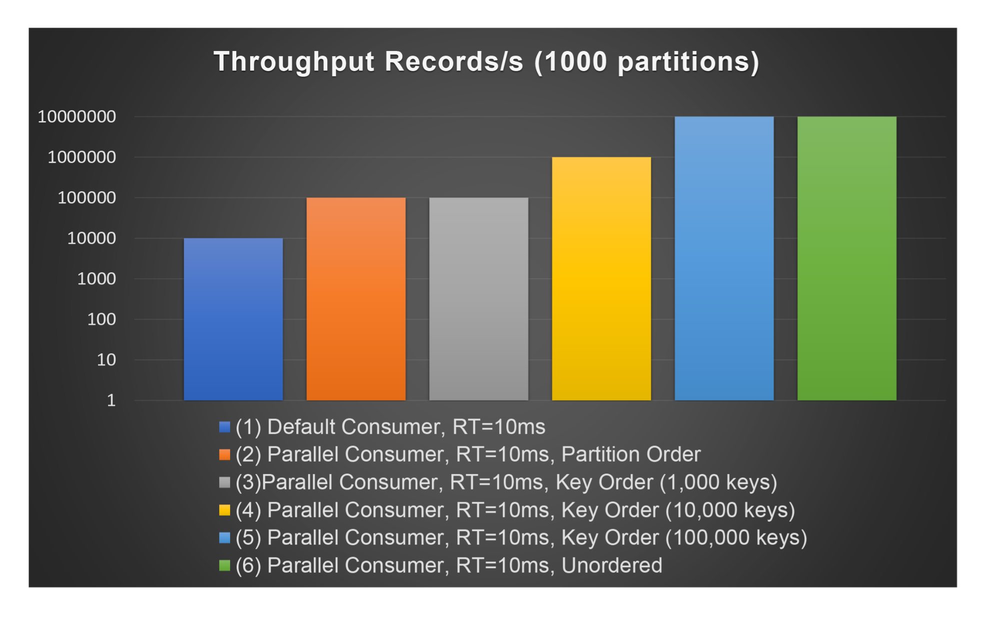
Note that all other things being equal, the throughput of the Key and Unordered modes will be highest and identical, if there are more keys than the concurrency of the consumers (number of consumers x threads per consumer) for the Key mode.  Of course, if there are less keys then the concurrency will be restricted, and throughput will be limited. For example, with only 1000 keys then the throughput of Key ordering is capped at 100,000 TPS (1000/0.01), which is less than the target throughput. The only solution then would be to use Unordered processing to achieve 1M TPS. 

On the other hand, the Unordered mode has essentially unlimited throughput, being limited in practice by the partition throughput and the resources for the consumers (consumers and number of threads per consumer)

Finally, just to show the potential improvement in throughput for each mode (and the limiting cases of the Key mode), if we increase the number of partitions to 1,000 (enabling a maximum throughput of 10M TPS for the topic), and allowing a maximum of 100 consumers (which only impacts the default consumer), then this example shows an increase in throughput of an order of magnitude from worst to best case (10,000 TPS to 10M TPS), and the impact of different key sizes (3-5): 

4. What Else?

There’s support for 2 other approaches to record processing that don’t use an explicit thread pool, Vert.x (from Eclipse—still my IDE of choice after Emacs and then Borland’s JBuilder which was killed off by Eclipse) and Reactor, actually part of the Spring framework.  Both use asynchronous, non-blocking processing to achieve potentially higher concurrency than explicit threadpools. Here’s an example of using Vert.x for remote HTTP calls, and a Reactor example.   Using either of these would invalidate my assumptions for the modeling done above (which all assumed explicit thread pool limits, although mostly for Unordered as the other modes all have concurrency constraints due to ordering over Partition or Key), so you’d have to run some benchmarks to get accurate throughput results. But just remember that on the Kafka cluster side the limiting factor is the number of partitions, and too many partitions are likely to actually start reducing the throughput.

There are also some other extras, including support for retries, batching (which is useful for sink systems such as OpenSearch which benefit from sending batches of documents at once), and choices for how to do offset commits. The best documentation for these and other options is probably in the code itself (yet another advantage of open source software). 

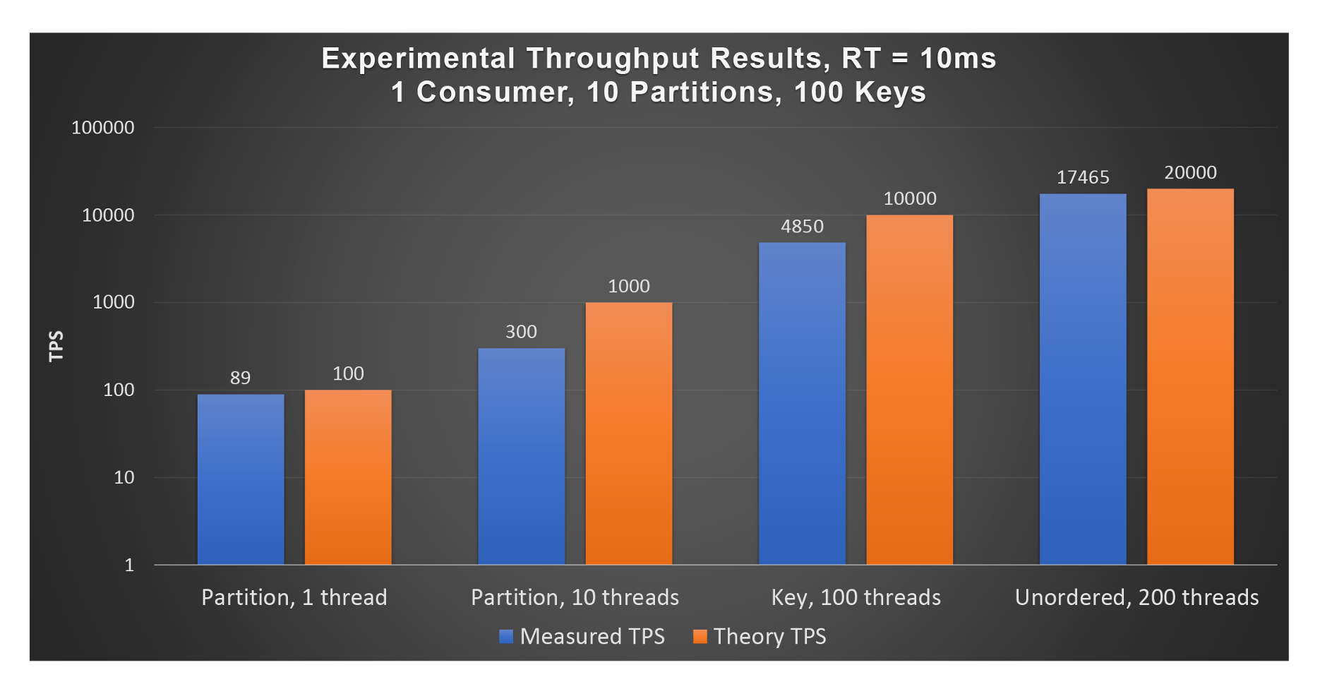
5. Experimental Results

Finally, just to confirm that everything works as advertised, I did some basic performance tests with a single consumer and topic with 10 partitions, 100 keys, and a constant record processing latency of 10ms. The version of Kafka was 3.1.1, and everything was running on a laptop (consumer only running, replaying data in topic). This graph (logarithmic y-axis) shows the consumer throughput obtained (blue) compared with the theory (orange) for various modes and consumer threads including Partition (1 thread, comparable to the default consumer), Partition (10 threads), Key (100 threads), and Unordered (200 threads), with results ranging from 89 TPS to 17,465 TPS. These gave a speedup over the default consumer throughput of 3.3, 54, and 196 times. The Unordered results are very close to predicted, but the Partition and Key results aren’t as good as expected. This was possibly due to some issues I detected with the unequal distribution of records from all the available Partitions (even though the consumer was allocated all 10 partitions, some polls did not appear to read from all partitions equally—some tuning of the poll size may have helped).  

6. Should You Use the Kafka Parallel Consumer?

From both theoretical and practical perspectives, the Kafka Parallel Consumer has the potential to significantly maximize consumer concurrency with fewer partitions, and therefore increase throughput and reduce latency, particularly with slow record processing. However, it is worth noting that it’s only up to version 0.5, and I discovered that it doesn’t support many of the methods that the default consumer does—or example, manual partition assignment and discovering what partitions are assigned to the consumer. It’s therefore not a direct drop-in replacement for the default consumer, but worth checking out for development and pre-production, however it may be worth waiting until version 1 before using it in production.

Here’s a final photo of the Jacquard loom (which actually has 2 Jacquard mechanisms, similar to 2 Kafka partitions – the photo on the museum website shows them), showing the benefits of parallel thread processing to make 18 ribbons concurrently.

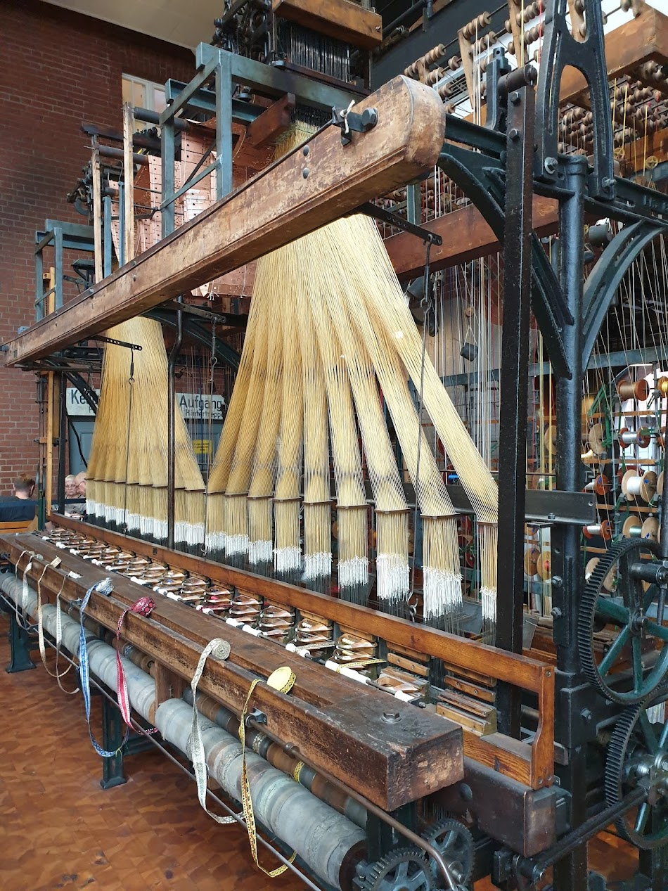
(Source: Paul Brebner)