


In the fourth blog of the “Around the World ” series we built a prototype of the application, designed to run in two georegions.
Recently I re-watched “Star Trek: The Motion Picture” (The original 1979 Star Trek Film). I’d forgotten how much like “2001: A Space Odyssey” the vibe was (a drawn out quest to encounter a distant, but rapidly approaching very powerful and dangerous alien called “V’ger”), and also that the “alien” was originally from Earth and returning in search of “the Creator”—V’ger was actually a seriously upgraded Voyager spacecraft!

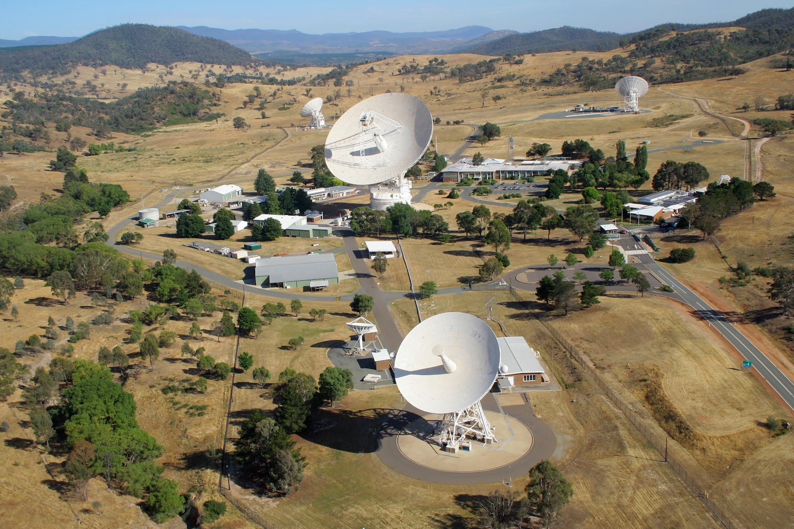
The original Voyager 1 and 2 had only been recently launched when the movie came out, and were responsible for some remarkable discoveries (including the famous “Death Star” image of Saturn’s moon Mimas, taken in 1980). Voyager 1 has now traveled further than any other human artefact and has since left the solar system! It’s amazing that after 40+ years it’s still working, although communicating with it now takes a whopping 40 hours in round-trip latency (which happens via the Deep Space Network—one of the stations is at Tidbinbilla, near our Canberra office).
Luckily we are only interested in traveling “Around the World” in this blog series, so the latency challenges we face in deploying a globally distributed stock trading application are substantially less than the 40 hours latency to outer space and back. In Part 4 of this blog series we catch up with Phileas Fogg and Passepartout in their journey, and explore the initial results from a prototype application deployed in two locations, Sydney and North Virginia.
1. The Story So Far
In Part 1 of this blog series we built a map of the world to take into account inter-region AWS latencies, and identified some “georegions” that enabled sub 100ms latency between AWS regions within the same georegion. In Part 2 we conducted some experiments to understand how to configure multi-DC Cassandra clusters and use java clients, and measured latencies from Sydney to North Virginia. In Part 3 we explored the design for a globally distributed stock broker application, and built a simulation and got some indicative latency predictions.
The goal of the application is to ensure that stock trades are done as close as possible to the stock exchanges the stocks are listed on, to reduce the latency between receiving a stock ticker update, checking the conditions for a stock order, and initiating a trade if the conditions are met.
2. The Prototype
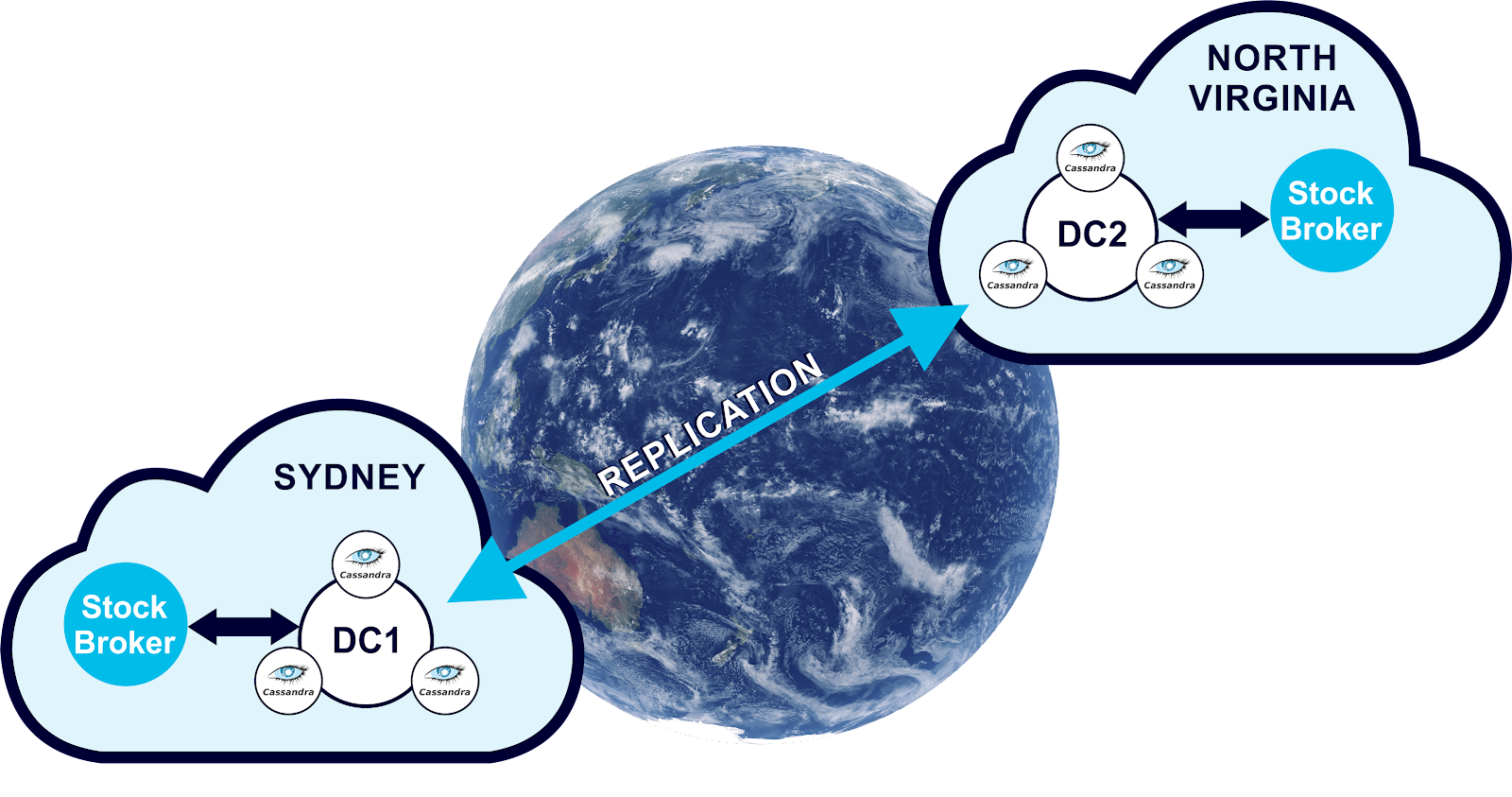
For this blog I built a prototype of the application, designed to run in two georegions, Australia and the USA. We are initially only trading stocks available from stock exchanges in these two georegions, and orders for stocks traded in New York will be directed to a Broker deployed in the AWS North Virginia region, and orders for stocks traded in Sydney will be directed to a Broker deployed in the AWS Sydney region. As this Google Earth image shows, they are close to being antipodes (diametrically opposite each other, at 15,500 km apart, so pretty much satisfy the definition of traveling “Around the World”), with a measured inter-region latency (from blog 2) of 230ms.

The design of the initial (simulated) version of the application was changed in a couple of ways to:
- Ensure that it worked correctly when instances of the Broker were deployed in multiple AWS regions
- Measure actual rather than simulated latencies, and
- Use a multi-DC Cassandra Cluster.
The prototype isn’t a complete implementation of the application yet. In particular it only uses a single Cassandra table for Orders—to ensure that Orders are made available in both georegions, and can be matched against incoming stock tickers by the Broker deployed in that region.
Some other parts of the application are “stubs”, including the Stock Ticker component (which will eventually use Kafka), and checks/updates of Holdings and generation of Transactions records (which will eventually also be Cassandra tables). Currently only the asynchronous, non-market, order types are implemented (Limit and Stop orders), as I realized that implementing Market orders (which are required to be traded immediately) using a Cassandra table would result in too many tombstones being produced—as each order is deleted immediately upon being filled (rather than being marked as “filled” in the original design, to enable the Cassandra query to quickly find unfilled orders and prevent the Orders table from growing indefinitely). However, for non-market orders it is a reasonable design choice to use a Cassandra table, as Orders may exist for extended periods of time (hours, days, or even weeks) before being traded, and as there is only a small number of successful trades (10s to 100s) per second relative to the total number of waiting Orders (potentially millions), the number of deletions, and therefore tombstones, will be acceptable.
We now have a look at the details of some of the more significant changes that were made to the application.
Cassandra
I created a multi-DC Cassandra keyspace as follows:
1 | CREATE KEYSPACE broker WITH replication = {'class': 'NetworkTopologyStrategy', 'NorthVirginiaDC': '3', 'SydneyDC': '3'}; |
In the Cassandra Java driver, the application.conf file determines which Data Center the Java client connects to. For example, to connect to the SydneyDC the file has the following settings:
1 2 3 4 5 6 7 8 9 10 11 | datastax-java-driver { basic.contact-points = [ "1.2.3.4:9042" ] basic.load-balancing-policy { class = DefaultLoadBalancingPolicy local-datacenter = "SydneyDC" } } |
The Orders table was created as follows (note that I couldn’t use “limit” for a column name as it’s a reserved word in Cassandra!):
1 2 3 4 5 6 7 8 9 10 11 12 13 | CREATE TABLE broker.orders ( symbol text, orderid text, buyorsell text, customerid text, limitthreshold double, location text, ordertype text, quantity bigint, starttime bigint, PRIMARY KEY (symbol, orderid) ); |
For the primary key, the partition key is the stock symbol, so that all outstanding orders for a stock can be found when each stock ticker is received by the Broker, and the clustering column is the (unique) orderid, so that multiple orders for the same symbol can be written and read, and a specific order (for an orderid) can be deleted. In a production environment using a single stock symbol partition may result in skewed and unbounded partitions which is not recommended.
The prepared statements for creating, reading, and deleting orders are as follows:
1 2 3 4 5 6 7 8 9 | PreparedStatement prepared_insert = Cassandra.session.prepare( "insert into broker.orders (symbol, orderid, buyorsell, customerid, limitthreshold, location, ordertype, quantity, starttime) values (?, ?, ?, ?, ?, ?, ?, ?, ?)"); PreparedStatement prepared_select = Cassandra.session.prepare( "select * from broker.orders where symbol = ?"); PreparedStatement prepared_delete = Cassandra.session.prepare( "delete from broker.orders where symbol = ? and orderid = ?"); |
I implemented a simplified “Place limit or stop order” operation (see Part 3), which uses the prepared_insert statement to create each new order, initially in the Cassandra Data Center local to the Broker where the order was created from, which is then automatically replicated in the other Cassandra Data Center. I also implemented the “Trade Matching Order” operation (Part 3), which uses the prepared_select statement to query orders matching each incoming Stock Ticker, checks the rules, and then if a trade is filled deletes the order.
Deployment
I created a 3 node Cassandra cluster in the Sydney AWS region, and then added another identical Data Center in the North Virginia AWS regions using Instaclustr Managed Cassandra for AWS. This gave me 6 nodes in total, running on t3.small instances (5 GB SSD, 2GB RAM, 2 CPU Cores). This is a small developer sized cluster, but is adequate for a prototype, and very affordable (2 cents an hour per node for AWS costs) given that the Brokers are currently only single threaded so don’t produce much load. We’re more interested in latency at this point of the experiment, and we may want to increase the number of Data Centers in the future. I also spun up an EC2 instance (t3a.micro) in the same AWS regions, and deployed an instance of the Stock Broker on each (it only used 20% CPU). Here’s what the complete deployment looks like:
3. The Results
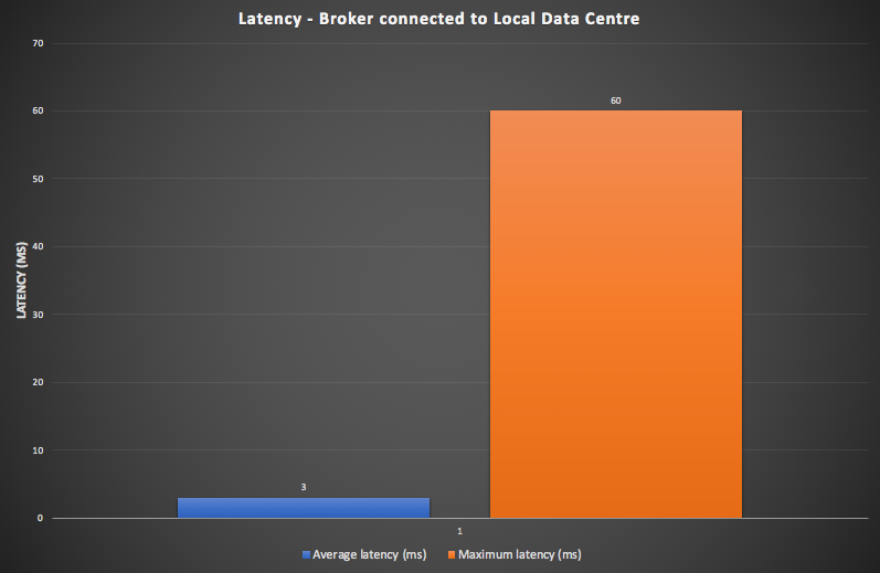
For the prototype, the focus was on demonstrating that the design goal of minimizing latency for trading stop and limit orders (asynchronous trades) was achieved. For the prototype, the latency for these order types is measured from the time of receiving a Stock Ticker, to the time an Order is filled. We ran a Broker in each AWS region concurrently for an hour, with the same workload for each, and measured the average and maximum latencies. For the first configuration, each Broker is connected to its local Cassandra Data Center, which is how it would be configured in practice. The results were encouraging, with an average latency of 3ms, and a maximum of 60ms, as shown in this graph.
During the run, across both Brokers, 300 new orders were created each second, 600 stock tickers were received each second, and 200 trades were carried out each second.
Given that I hadn’t implemented Market Orders yet, I wondered how I could configure and approximately measure the expected latency for these synchronous order types between different regions (i.e. Sydney and North Virginia)? The latency for Market orders in the same region will be comparable to the non-market orders. The solution turned out to be simple— just re-configure the Brokers to use the remote Cassandra Data Center, which introduces the inter-region round-trip latency which would also be encountered with Market Orders placed on one region and traded immediately in the other region. I could also have achieved a similar result by changing the consistency level to EACH_QUOROM (which requires a majority of nodes in each data center to respond). Not surprisingly, the latencies were higher, rising to 360ms average, and 1200ms maximum, as shown in this graph with both configurations (Stop and Limit Orders on the left, and Market Orders on the right):
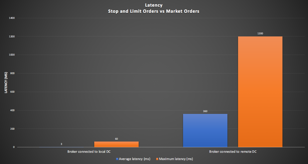
So our initial experiments are a success, and validate the primary design goal, as asynchronous stop and limit Orders can be traded with low latency from the Broker nearest the relevant stock exchanges, while synchronous Market Orders will take significantly longer due to inter-region latency.
Write Amplification
I wondered what else can be learned from running this experiment? We can understand more about resource utilization in multi-DC Cassandra clusters. Using the Instaclustr Cassandra Console, I monitored the CPU Utilization on each of the nodes in the cluster, initially with only one Data Center and one Broker, and then with two Data Centers and a single Broker, and then both Brokers running. It turns out that the read load results in 20% CPU Utilization on each node in the local Cassandra Data Center, and the write load also results in 20% locally. Thus, for a single Data Center cluster the total load is 40% CPU. However, with two Data Centers things get more complex due to the replication of the local write loads to each other Data Center. This is also called “Write Amplification”.
The following table shows the measured total load for 1 and 2 Data Centers, and predicted load for up to 8 Data Centers, showing that for more than 3 Data Centers you need bigger nodes (or bigger clusters). A four CPU Core node instance type would be adequate for 7 Data Centers, and would result in about 80% CPU Utilization.
| Number of Data Centres | Local Read Load | Local Write Load | Remote Write Load | Total Write Load | Total Load |
| 1 | 20 | 20 | 0 | 20 | 40 |
| 2 | 20 | 20 | 20 | 40 | 60 |
| 3 | 20 | 20 | 40 | 60 | 80 |
| 4 | 20 | 20 | 60 | 80 | 100 |
| 5 | 20 | 20 | 80 | 100 | 120 |
| 6 | 20 | 20 | 100 | 120 | 140 |
| 7 | 20 | 20 | 120 | 140 | 160 |
| 8 | 20 | 20 | 140 | 160 | 180 |
Costs
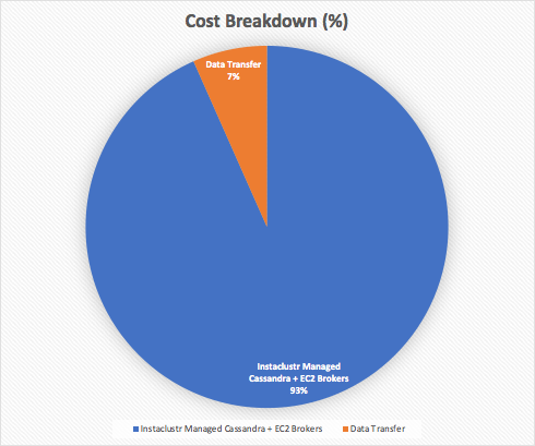
The total cost to run the prototype includes the Instaclustr Managed Cassandra nodes (3 nodes per Data Center x 2 Data Centers = 6 nodes), the two AWS EC2 Broker instances, and the data transfer between regions (AWS only charges for data out of a region, not in, but the prices vary depending on the source region). For example, data transfer out of North Virginia is 2 cents/GB, but Sydney is more expensive at 9.8 cents/GB. I computed the total monthly operating cost to be $361 for this configuration, broken down into $337/month (93%) for Cassandra and EC2 instances, and $24/month (7%) for data transfer, to process around 500 million stock trades. Note that this is only a small prototype configuration, but can easily be scaled for higher throughputs (with incrementally and proportionally increasing costs).
Conclusions
In this blog we built and experimented with a prototype of the globally distributed stock broker application, focussing on testing the multi-DC Cassandra part of the system which enabled us to significantly reduce the impact of planetary scale latencies (from seconds to low milliseconds) and ensure greater redundancy (across multiple AWS regions), for the real-time stock trading function. Some parts of the application remain as stubs, and in future blogs I aim to replace them with suitable functionality (e.g. streaming, analytics) and non-functionality (e.g. failover) from a selection of Kafka, Elasticsearch and maybe even Redis!