
Image from NASA’s James Webb Space Telescope showing thousands of galaxy clusters (https://webbtelescope.org/contents/media/images/2022/038/01G7JGTH21B5GN9VCYAHBXKSD1?news=true) public domain
Recently I decided to take a closer look at the cloud computing clusters that Instaclustr uses to provide managed open source Big Data services to 100s of customers, to see if I could discover any interesting resource and performance/scalability insights. I plan to examine a variety of cluster data that we have available, including the number and size of clusters and performance metrics.
In this first part, I will focus on the number and size of clusters and reveal some discoveries about the nature of scalability in Apache Cassandra®, Apache Kafka®, OpenSearch® (and other) technologies.
1. What’s in the Data?
The raw data consists of information about each production and non-production cluster in our managed cloud fleet on a particular date in the recent past. It includes the cluster size (number of nodes—a node is a cloud provider instance—e.g., AWS EC2 instance), the node sizes (the cloud provider specific instance type used in the cluster), and the number of data centres (some of the bigger clusters are deployed to multiple cloud provider DCs, up to 6). The technologies include Apache Cassandra, Apache Kafka, Kafka® Connect, Apache ZooKeeper™, Elasticsearch/OpenSearch®, Redis™, PostgreSQL®, and Cadence®.
In theory, a more accurate representation of the cluster size is the number of nodes multiplied by the number vCPUs in each node, but for simplicity, I’ve only used the number of nodes to start with.
Most of these technologies are horizontally scalable, which means that the cluster capacity can be increased by adding more nodes. However, the “replication factor” used in production clusters is typically “3”, which means that the minimum size of clusters is 3 nodes, and that clusters are often scaled out in increments of 3. There is also a theory that clusters should have an odd number of nodes (e.g. to ensure that the quorum protocol works correctly), but in practice they can have an even number of nodes.
Instaclustr allows for vertical scaling of Cassandra and Kafka—for vertical scaling, cluster capacity is increased without an increase in the number of nodes (horizontal scaling, on the other hand, increases the number of nodes).
First, I computed some basic statistics.
The maximum cluster size is MaxSize nodes (where MaxSize is > 100). The minimum size is 1 (non-production clusters), the median is 3, but the average is 7.2. This implies that the distribution is skewed, but by how much? The standard deviation is 20, which also implies a wide range of cluster sizes. The largest clusters are dominated by Apache Cassandra, with Apache Kafka coming in 2nd.
First, let’s just take a look at the raw data—cluster size, in order of decreasing cluster size (we have normalized the nodes for cluster, with 1 being the largest cluster).
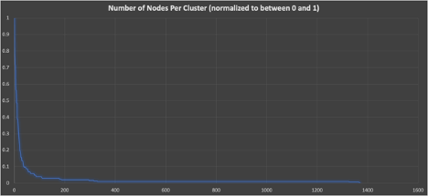
Graph 1
This confirms the statistics, cluster size is a long-tailed distribution with few large clusters, and many smaller clusters. Next, let’s take a look at the cumulative distribution function— this plots the normalized cluster size on the x-axis (0-1) vs the percentage (out of 100%) on the y-axis that are less than or equal to the size.
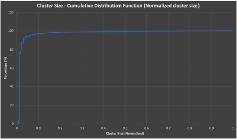
Graph 2
What does this tell us? That 80% of clusters are less than or equal to 6 nodes in size. 87% are less than or equal to 9 nodes in size—only 3% are greater than 9 nodes in size (computed using un-normalized cluster sizes).
Here’s the same data as Graph 1, but this time ordered by increasing normalized cluster size (to enable easier comparison with some alternative distributions):
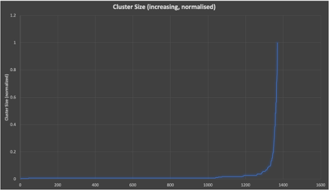
Graph 3
Graphs 1 to 3 tell us that the cluster size distribution is not something more “normal” like a uniform or normal distribution.
If the distribution was uniform, then cluster sizes ordered by increasing size would look like this (although the average cluster size would then be far higher than observed):
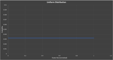
Graph 4
And if the distribution was normal (well, sort of normal, it’s a skewed normal distribution, as I’ve forced it to have the observed average of 7.2), here’s what the distribution of cluster sizes would look like (x-axis is cluster, y is probability):
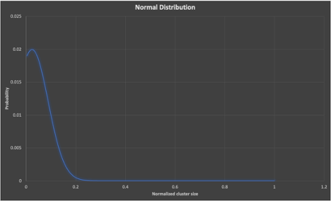
Graph 5
So, if they aren’t uniform or normal, what distribution could the cluster sizes be?
2. What is Zipf’s Law?

Elephants are a lot heavier than the next biggest animal—and so on (Source: Shutterstock)
Zipf’s law is a common rank-size distribution function, or scaling law, that was originally observed for the frequency of words in a language—it often fits “stretched” exponential distributions similar to our cluster data. It describes the fact that the most common word occurs approximately twice as often as the next most common word, 3 times as often as the third most common word, and so on (frequency is 1/Rank). Zipf’s law can be graphed by plotting the frequency data on a log-log graph, the log of rank order against the log of frequency, giving an approximately linear function.
Here’s an example graph showing Zipf’s law for Wikipedia words in different languages.
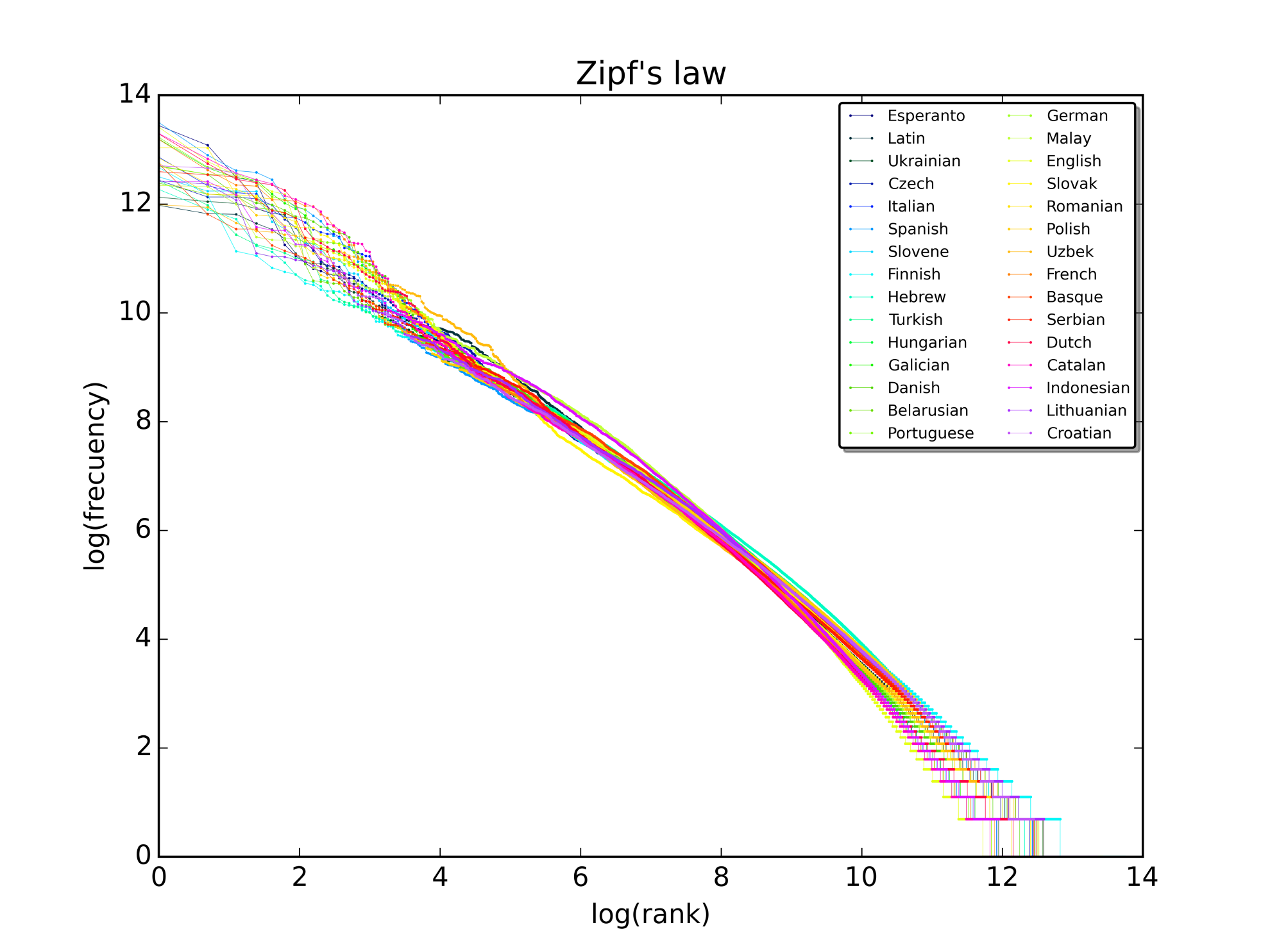
A plot of the rank versus frequency for the first 10 million words in 30 Wikipedia’s in a log-log scale. (Source: https://commons.wikimedia.org/wiki/File:Zipf_30wiki_en_labels.png)
It turns out that Zipf’s law holds (at least approximately, or for a subset of the observations) for a variety of other things, both artificial and natural, including cities, wealth distribution, animal species, galaxy cluster sizes, earthquakes, lunar craters, and even computer systems (e.g., search, data compression, workloads, resources, etc.). It’s not always exact, but when it’s not, it can reveal interesting errors about the underlying data. For example, there are deviations for cities due to the fact that some cities merge with other nearby cities (aggregation), arbitrary postcodes, and geographical and political constraints etc. There have been numerous attempts to explain the underlying mechanisms resulting in Zipf’s law, but the simplest is along the lines of “the rich get richer”—for cities, this means that bigger cities attract more people faster than smaller cities.
Let’s see what Zipf’s law looks like for the Instaclustr cluster data. This graph shows log of cluster size vs. log of cluster rank.
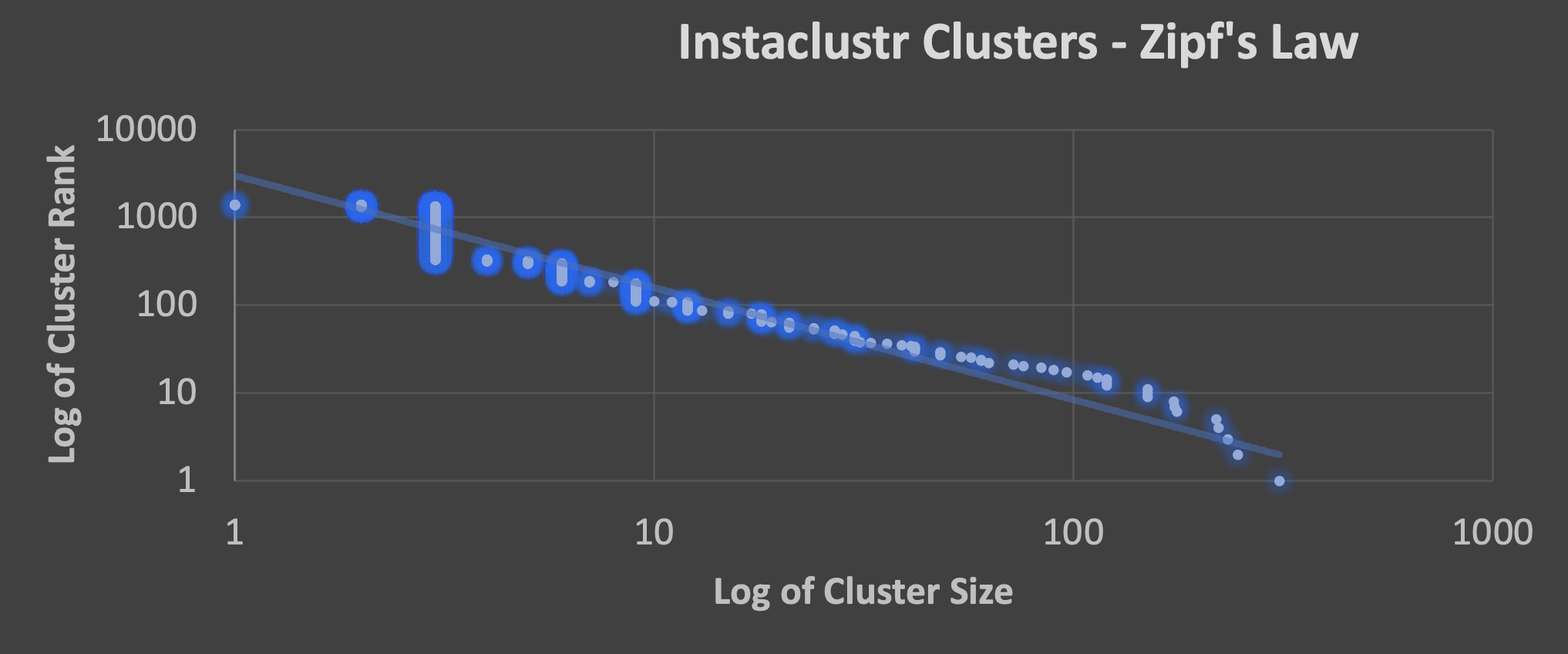
Graph 6
The distribution certainly looks reasonably Zipfian (the solid line is the ideal Zipfian distribution), with a few differences. For example:
- there are some “clumps” resulting from a large number of clusters of the same size (e.g., 3, 6, and 9 nodes)
- the single node clusters are anomalous and fall below the theoretical line (and could probably be excluded from the data set, as they don’t really count as “clusters”)
- from around 42 nodes the clusters diverge (being increasingly above the line—indicating they are bigger than predicted—maybe because horizontally scalable systems tend to be more expensive for smaller systems—they have more upfront overheads—but become more efficient the bigger they get)
- But from around 200 nodes they drop below the line (indicating that they are smaller than predicted). In fact, extrapolating the theoretical line forwards until it hits the x-axis, results in a prediction of the biggest cluster size being larger, in excess of 500 nodes.
3. Insights into Instaclustr’s Clusters from Zipf’s Law
Let’s see what Zipf’s law can potentially tell us about our clusters.
3.1 Bigger Clusters

Maraapunisaurus dinosaurs were giant herbivores! (Source: Creative Commons Attribution-Share Alike 4.0)
For systems that follow Zipf’s law, it predicts that there is the potential for even larger observations—in our example, that means potentially bigger clusters (c.f. unseen galaxies—and extinct animal species, e.g., the biggest dinosaur ever was Maraapunisaurus weighing an estimated 150 tonne). Zipf’s law also predicted that bigger galaxies would be detected in older parts of the universe (beyond the reach of the Hubble at the time), and their existence was confirmed recently with the release of the James Webb telescope observations (see the initial image above).
So, it’s likely that at some point in the future, we’ll see even bigger clusters in our fleet of managed services. For example, Cassandra v4.0 is more scalable than ever, and now that Kafka has abandoned ZooKeeper and replaced it with an internal Kafka Raft protocol (KRaft), bigger Kafka clusters are entirely possible.
3.2 Total Number of Nodes

Two Lions is about the limit for this vehicle (Source: Getty Images)
One clever trick with Zipf’s law is if you know the size of the largest observation, you can estimate the total size of the system. So, if you know the size of the biggest cluster, we can estimate the total number of nodes needed for all clusters. Zipf’s law also implies that as the number of observations increases, the total size of the system increases slower (and actually tends to an upper limit). Let’s see how this works for a different example, transporting representative samples of many animal species. We assume that elephants are the biggest species (whales are not welcome). How can a zookeeper fit 100s of animal species in a finite space in a truck? Essentially, most species don’t really weigh much.
Here’s the graph for the total weight of animals to be transported (in tonnes). The first 200 species get you to 70 tonnes, but by 1000 species this adds only another 20 tonnes (90 in total—well within the capacity of a 175 tonne Australian “road train” truck!).
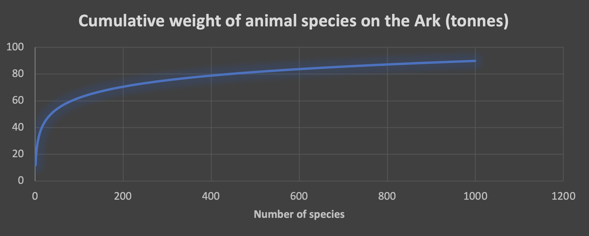
Graph 7
For clusters, this isn’t exact as you can’t have clusters with less than 1 node, but the general rule applies—doubling the total number of clusters will only increase the total nodes by significantly less than a factor of 2, and the total number of nodes in all clusters will tend to a limit as the number of clusters increases.
For example, if we expect to double the number of clusters in 12 months’ time, with the largest cluster expanded to 1,000 nodes, the total number of nodes in all the clusters is approximately 45% more.
This could be useful for planning expected revenue/cost growth, to ensure sufficient instance types overall or for specific cloud regions, etc.
3.3 Less Large Clusters, More Small Clusters
Zipf’s law predicts that there will be fewer large clusters, but a lot more small clusters. From our data, we can see this, as the top 10 clusters have 20% of the total nodes, and the top 20 have 30% of the total nodes. In terms of cluster resourcing and management, this implies that a relatively small number of clusters will consume most resources and probably grow bigger over time.
Zipf’s law also predicts lots of smaller clusters, as it typically predicts a longer tail than other exponential distributions. Countries have lots of very small towns, a few online retailers can benefit from selling lots of “odd” things that traditional shops can’t afford to stock (see Tale of Tails), etc. In terms of clusters, lots of customers will only want small clusters. Why is this? Common use cases for small clusters include free trials, small development and test clusters, customer who are small start-ups (but hope to grow bigger), and bigger customers wanting a larger number of small clusters rather than a single big cluster (this is common for Kafka). It’s also possible that many customers choose horizontally scalable open source technologies because of the benefits and attraction of the open source ecosystem, rather than needing (at least initially) high throughput systems.
For our cluster data, the smallest 94% (and the biggest 6%) of the clusters have 50% of the total nodes.
3.4 Incremental Continuous Jumps in Cluster Sizes
The relatively incremental and continuous distribution of cluster sizes from 3 to MaxSize (rather than just a few size clumps, or big jumps in cluster sizes) tells us something about customer workloads and the ability of horizontally scalable cloud-hosted services to satisfy diverse workload requirements. The incremental continuous distribution of cluster sizes tells us that horizontal scaling “works”—it’s practical and affordable to have any cluster size you need, and the cluster sizes can be scaled horizontally to meet increasing workloads demands, incrementally—without having to over-resource clusters.
4. Why?
But why does the size of Instaclustr’s clusters follow Zipf’s law? In an attempt to find out, I watched the “The Zipf Mystery” (video), which explores several theories about why Zipf’s law works in general (for both artificial and natural systems). Several promising explanations include probability (the most common words are very short), laziness (The Principle of Least Effort), and power laws (“the rich get richer”). For computer clusters, some explanations are small clusters are easier to create, cheaper to run, and there are more use cases. Larger clusters are harder to create, cost more to run, and there are fewer use cases/workloads that fit larger clusters of specific sizes. However, they may tend to grow faster (and don’t contract) as:
- they can be expanded horizontally (only out), and vertically (up and down);
- large workloads may grow faster; and
- it may be easier to reuse an existing cluster for new use cases and applications that come along, thereby adding to the growth pressures on bigger clusters.
So, larger clusters are less frequent, but approximately follow the Zipfian distribution—that’s also why it pays to use a managed service for large clusters—larger clusters are often more mission-critical and you need someone you can trust managing them for you—check us out.
Further Reading
- A Tale of Tails
- Cities on Earth evolve in the same way as galaxies in space
- Zipf’s law for cosmic structures: How large are the greatest structures in the universe?
- Rethinking the Universe: Astronomers Disturbed by the Unexpected Scale of James Webb’s Galaxies
- Automatic Performance Modelling from Application Performance Management (APM) Data
- Performance Evaluation with Heavy Tailed Distributions
- The Zipf Mystery —cool video exploring why Zipf’s law may work (hint: for words it may just be probability!)