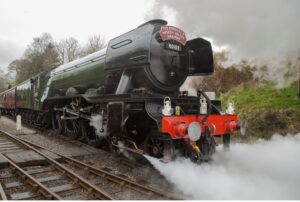
The Flying Scotsman was the first steam locomotive to break the 100 miles per hour speed record (161 km/h way back in 1934) (Source: Shutterstock) 

The Flying Scotsman was a 1900’s (in service 1923-1963) steam locomotive built for speed and scale—the steam era equivalent of Big Data cloud technologies today. It was big (100 tons, 21m long, 3 cylinders) and designed for non-stop runs of 631 km from London to Edinburgh (which required a larger tender with a corridor to allow a change of engine crew). It held many records including the first steam locomotive to reach 100 mph (161 km/h) in 1934, the longest non-stop run of 679 km (in Australia!), and when it retired it had covered over 2 million miles.  

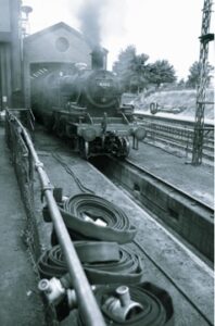
But steam locomotives were complex and dangerous machines. They had lots of moving parts, fireboxes, and high-pressure steam boilers. Engine cabs had myriads of pipes, levers, and dials which the drivers had to pay careful attention to—to arrive on schedule, without wasting coal or water, and without exploding the boiler. 

(Source: https://www.thelondoneconomic.com/travel/fascinating-photos-show-inner-engine-flying-scotsman-47402/)

Like a steam locomotive, Apache Kafka also has lots of “moving parts”. A Kafka cluster is actually a distributed system, a cluster, which consists of multiple brokers (servers)—messages are sent to Kafka with producers, and consumers receive messages. Topics are used to direct messages between producers and consumers—producers write to selected topics, and consumers subscribe and read from selected topics. Topics are divided up into partitions, and the partitions are distributed over the available brokers for high availability and concurrency. Partitions are replicated to other partitions (followers) from the leader partition (3 is common for production clusters).  

 Here’s a Kafka UML diagram that has been reused many times (from one of my early Kafka blogs).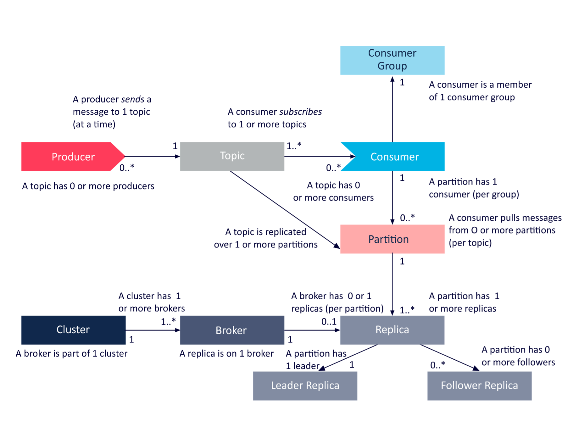 

But from a train passenger’s perspective, the only dial that matters is the speedometer (the one in the middle below)—as that determines if they get home in time for dinner. 

Speedometer from the ‘W’ Class Locomotive “Malcolm Moore” on display at Broken Hill, NSW (Source: Paul Brebner)

It may come as a surprise that most steam locomotives didn’t come with a speedometer. It was up to the driver to manually determine their speed. But some express passenger trains had a speedometer in the first-class carriages for the convenience of the passengers! 

Let’s take a look at some of the Apache Kafka metrics available in the console of Instaclustr’s Managed Kafka service (the “dials” for Kafka) which are most relevant to Kafka developers.    

First, are there metrics that tell us how fast we are traveling—a speedometer? For computer systems in general, these would typically be rate metrics—the number of things occurring over some period of time. For Apache Kafka, this is equivalent to the Kafka cluster message throughout—the rate of messages going into and then coming out of the cluster—that is, the cluster workload. 

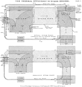
Sankey Diagrams are an excellent visual representation of flow between systems – they were used to describe steam engines in 1898!  

(Source: Ciminieri, Daniele & Menard, Raphael & Meunier, Guillaume & Ciuccarelli, Paolo. (2014). Energetical streams visualization using interactive Sankey diagrams. 10.13140/RG.2.1.2490.0886.) 

Below is a simple Sankey Diagram showing example flow rates (from producers on the left to consumers on the right) in and out of the Kafka cluster for a steady state system with 90 messages/s flowing in, and the same flowing out. 

Cluster-level view of message flow 

1. Broker Topic Metrics 

The console provides high-level (aggregated across all topics) Kafka Broker -> Broker Topics Metrics graphs (support documentation here). The available graphs are Broker Topic Bytes In (per second), Broker Topic Bytes Out (per second), and Broker Topic Messages In (per second). The one-minute rate graphs are the most useful, and display a per-second rate (averaged over the past minute, so they may take up to a minute to respond to changes).  They show the total bytes and message rate for all topics for each Kafka broker (which is identified by an IP address).  

However, to get the total byte/message rate for the Kafka cluster you have to sum the individual broker rates. For example, for a 3 broker cluster, and “Messages In: One Minute Rate” of 30 per broker, the total cluster Messages In rate is 30 x 3 = 90 messages/s (assuming an equal rate per broker, which is not always the case). 

Here’s a Sankey Diagram showing what’s going on with a flow rate from a Producer/s (90/s), a total Messages In rate to the cluster of 90/s, split across 3 brokers (30/s each), and a total Messages Out rate of 90/s resulting from a single consumer group. 

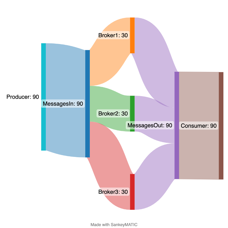
Broker level view of message flow 

Note that the Broker Topic Messages In rate corresponds to the Apache Kafka documented “Message in rate” metric with the MBean (with ‘topic=’ omitted yielding the all-topic rate): 

The Broker Topic Bytes In rate corresponds to the “Byte in rate from clients” (omitting ‘topic=’) with the MBean: 

And Broker Topic Byes Out rate corresponds to the “Byte out rate to clients” (again with no ‘topic=’) and the MBean: 

You can compute the average message size from the “Broker Topic Bytes In: One Minute Rate” graph. For example, if this graph shows 300 bytes per node, giving a total of 900 bytes per second for the cluster, then the message size is 900/90 = 10 bytes per message on average.  

There is no Messages Out rate (as Kafka doesn’t provide it), but there is a “Broker Topic Bytes Out: One Minute Rate” graph. If this shows 0 then no consumers are subscribed to the topics. If it shows a non-zero value, then consumers are running. Depending on how many consumers groups are subscribed to topics, the out rate can be higher than the in rate.  

The non-existent average Messages Out rate can be computed from the computed input message size as: 

Messages Out rate = Broker Topic Bytes Out: One Minute Rate/Average input message size = 900/10 = 90 messages/s. 

This assumes a steady state flow of messages in and out of Kafka with a single consumer group. If there are multiple consumer groups, then the output message rate can be higher than the input rate. For example, with 2 consumer groups, and Bytes Out rate of 1,800, then: 

Messages out rate = 1800/10 = 180 messages/s. 

This Sankey Diagram illustrates this with two consumer groups receiving the same messages, thereby doubling the output rate.  

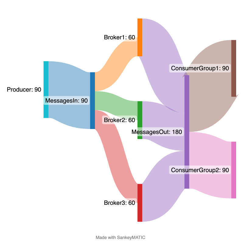
Broker level view of message flow, with two consumer groups 

2. Per-Topic Metrics 

A cutaway view of a steam locomotive showing the superheater tubes (Source: Parrot of Doom, CC BY-SA 3.0, via Wikimedia Commons)

Steam locomotives have lots of superheater steam tubes—Kafka has lots of topics! 

We also provide the more detailed version of these metrics, per-topic metrics, under “Kafka Topics” -> Message In/Byte In/Out. These are the same metrics as above but for a single selected topic. Again, there is no Message Out rate, but it can be computed in the same way from Byte In/Out. 

Note that computing the rate sums and Message Out rate can be automated if you are using our monitoring API in conjunction with Grafana and Prometheus (Here’s a previous blog on this topic, and our Prometheus support pages). 

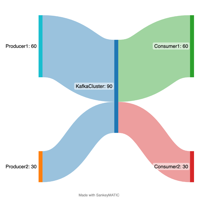
This Sankey Diagram shows the more detailed per topic/per broker story with 2 producers, 2 topics and 2 consumer groups (assuming producer1 sends to topic1 and consumer1 reads from topic1. 

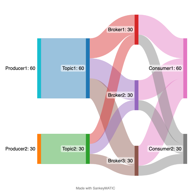
Broker/topic level view of message flow. 

3. Consumer Group Metrics 

Steam locomotives often used sand to reduce wheel slip (Source: Les Chatfield from Brighton, England, CC BY 2.0, via Wikimedia Commons) 

There’s another set of metrics for the output side of Kafka, the consumer groups. These are perhaps comparable to the cylinder pressure gauges in a steam locomotive which tells the driver how much steam is being taken from the boiler into the cylinders to provide motive power—apparently if you put too much pressure in too quickly the wheels would just spin and you would go nowhere—wheel slip! 

The next level of detail available is consumer group metrics, this is found under “Kafka Consumers” -> Consumer Group -> Metrics, and then Consumer Group Topics and Clients (i.e., consumer groups can be subscribed to > 1 topic, and the metrics are computed per client). Here’s the Apache Kafka documentation for Consumer Group Metrics. 

Note that we say per client, why not per consumer? Well, it turns out that we use the consumer client.id to identify clients. If this value is unique (which it typically is), then these metrics are computed per consumer. However, if all the consumers in a group share the same client.id (which apparently is possible, and may be used to impose quotas), then our metrics are computed across all the consumers and so are really consumer group metrics (i.e., total consumers in the group, total lag, and total partitions for the topic).  

We expose Consumer Count per Client, Consumer Lag per Client, and Partition Count per Client graphs on the console. 

“Consumer Lag per Client: message count” is the consumer lag for a topic/consumer (consumer lag is the difference between the last committed offset by a consumer and the offset at the end for a particular partition). This metric is useful as a proxy for consumer latency (which we don’t expose as a metric in the console). It will typically be > 1 (i.e., not 0), and can typically jump around in the 10s. A higher or increasing lag indicates that the consumers are not keeping up with the messages in rate to the topic. Solutions include increasing the number of consumers in the group (see the next metric) and speeding up slow consumers.  

“Consumer Lag per Client” is probably the Apache Kafka Consumer Fetch Metric kafka.consumer:type=consumer-fetch-manager-metrics,client-id=”{client-id}”: 

records-lag-max: The maximum lag in terms of number of records for any partition in this window.  

 “Partition Count per Client” corresponds to the Apache Kafka Consumer Group Metric/Attribute Name: 

assigned-partitions: The number of partitions currently assigned to this consumer 

If this number is > 1 for a consumer, then there is the potential to increase the number of consumers in the group to increase the concurrency and therefore the throughput of the group. If it’s 1 (for all consumers in the group), then you will need to increase the number of partitions for the topic before increasing the number of consumers. If there’s an imbalance between the partition count per consumer then this indicates that some consumers are having to do more work than others.  

4. Node (Broker) Operating System Metrics 

(Source: Shutterstock) 

As well as stoking the firebox, steam locomotive firemen had to watch some different gauges to the driver to ensure the safety and efficiency of the engine. These were related to resources, and included water (boiler water level gauges) and steam pressure (boiler steam pressure gauge). There are also some Kafka Node (broker) metrics that it’s worth keeping an eye on as you increase the throttle on a Kafka cluster! 

CPU Usage shows the percentage of the CPU being utilized per broker. As this approaches 80% or more you may notice an increase in end-to-end message latency, and a plateauing in throughput.  Horizontal or vertical scaling of the Kafka cluster well before this occurs is a good idea. 

CPU (detailed) provides more detailed CPU metrics. The most useful is “IOWait: %” which shows the time the CPU I/O thread is waiting to perform disk reads or writes. This is a percent, and it should be low. A high or increasing value indicates a disk bottleneck.  

Memory Available is the amount of spare RAM available per node (in MB). If this drops too much then it indicates you may need to increase the size of the brokers. 

An Ash Pit  (Source: Ben Salter from Wales, CC BY 2.0, via Wikimedia Commons)

Steam locomotives required lots of preparation and cleaning after use, including the Flying Scotsman. Because they were coal-fired steam engines, they produced lots of waste material (smoke and ash). Ash from the firebox had to be emptied out of their ashpans after every trip over an ash pit—basically garbage collection for trains!  

So how do you know if you still have sufficient memory or not? Kafka is written in Scala and runs on the JVM, so keeping track of garbage collection (GC) is a good idea as GC times will go up with increasing memory pressure. 2 metrics are available under “Kafka Broker” -> Kafka Garbage Collection (Old Generation and Young Generation)—if the GC times start increasing you may need more memory. 

Given that Kafka is a distributed streaming system (internally with a cluster of multiple brokers, and externally with producer and consumer clients), the network is also a critical resource. We provide Network in and Network out (bytes) metrics.   

Finally, Disk Usage (% Used and Disk Available: GiB, Disk Used: GiB) tells you how much of the available disk space is utilized and how much storage there is/used on the brokers.  

Other network and IO related metrics are Network and Request Handler Capacity under the “Kafka Broker” metrics. Network Processor Idle Percent (0 to 1) shows the time that Kafka’s network processor threads (responsible for reading and writing from/to Kafka clients) are idle—the value should be closer to 1 than 0.  Request Handler Idle Percent (0 to 1) shows the idle time for Kafka’s request hander threads which are responsible for disk IO (and should also be closer to 1 than 0). If they are closer to 0, then it’s probably time to increase the cluster capacity.  

So, there you have the main Apache Kafka metrics that are relevant for developers using one of our managed Kafka clusters—Broker Topic Metrics, Topic Metrics, Consumer Group Metrics, and Operating System Metrics. There are lots more metrics that are more relevant for Kafka operations, or useful if something goes wrong with the cluster. For example, there are a bunch of metrics for Kafka replication – find out more here.   

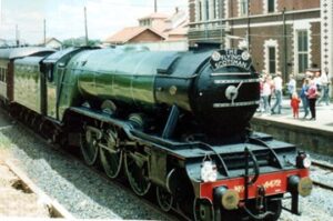
The Flying Scotsman in Australia in 1988/89 – it beat the longest non-stop run in the UK of 631km with a run of 679 km (Source: Zzrbiker at en.wikipedia, Public domain, via Wikimedia Commons)