In this second blog of “Around the World in (Approximately) 8 Data Centers” series we catch our first mode of transportation (Cassandra) and explore how it works to get us started on our journey to multiple destinations (Data Centers).

1. What Is a (Cassandra) Data Center?

What does a Data Center (DC) look like? Here are some cool examples of DCs (old and new)!

Arguably the first “electronic” data center was ENIAC, circa 1946, pictured below. It was, however, just a single (albeit monster) machine! It weighed more than 30 tonnes, occupied 1,800 square feet, consumed 200kW of power, got up to 50C inside, and was rumoured to cause blackouts in neighboring Philadelphia when it was switched on!

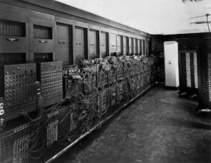
(Source: Shutterstock)

Jumping forward to the present, a photo of Google DC shows mainly cooling pipes. In common with ENIAC, power and heat are still a feature of modern DCs:

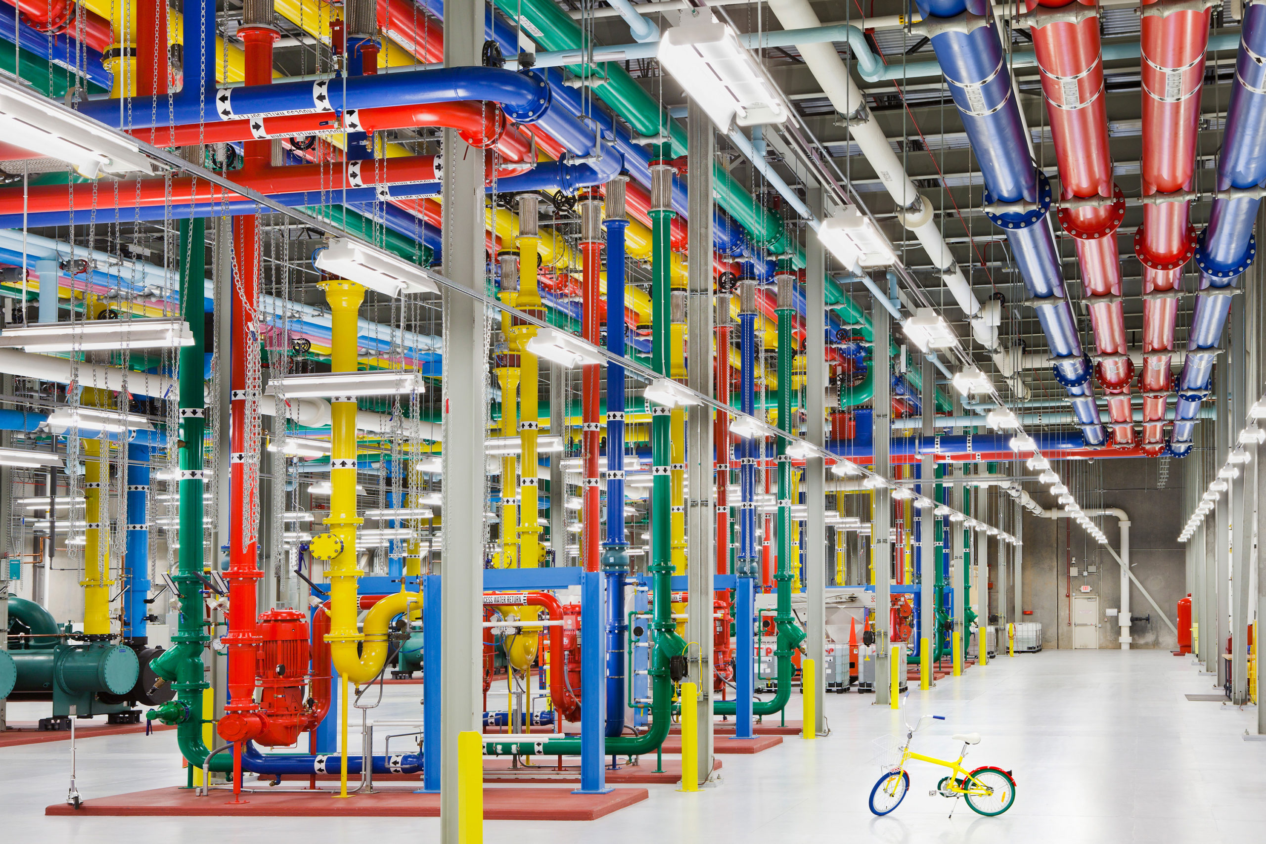
      (Source: www.google.com.au/about/datacenters/gallery/)

So what is a Cassandra Data Center?! Ever since I started using Cassandra I’ve been puzzled about Cassandra Data Centers (DCs). When you create a keyspace you typically also specify a DC name, for example:

The NetworkTopologyStrategy is a production ready replication strategy that allows you to have an explicit DC name. But why do you need an explicit DC name? The reason is that you can actually have more than one data center in a Cassandra Cluster, and each DC can have a different replication factor, for example, here’s an example with two DCs:

So what does having multiple DCs achieve? Powerful automatic global replication of data! Essentially you can easily create a globally distributed Cassandra cluster where data written to the local DC is asynchronously replicated to all the other DCs in the keyspace.  You can have multiple keyspaces with different DCs and replication factors depending on how many copies and where you want your data replicated to.

But where do the Cassandra DCs come from? Well, it’s easy to create a cluster in a given location and Data Center name in Instaclustr Managed Cassandra!

When creating a Cassandra cluster using the Instaclustr console, there is a section called “Data Center” where you can select from options including: 

Infrastructure Provider, Region, Custom Name, Data Center Network address block, Node Size, EBS Encryption option, Replication Factor, and number of nodes.

The Custom Name is a logical name you can choose for a data center within Cassandra, and is how you reference the data center when you create a keyspace with NetworkTopologyStrategy. 

So that explains the mystery of single Cassandra Data Center creation. What does this look like once it’s provisioned and running? Well, you can use CQLSH to connect to a node in the cluster, and then discover the data center you are connected to as follows:

How about multiple DCs?  Using Instaclustr Managed Cassandra the simplest way of creating multiple DC Cassandra clusters is to create a single DC cluster first (call it ‘DCHere’). Then in the management console for this cluster, click on “Add a DC”.  You can add one DC at a time to create a cluster with the total number of DCs you need, just follow our support documentation here and here.

2. Multi-Data Center Experiments With CQLSH

So, to better understand how Cassandra DCs work I created a test cluster with 3 nodes in each of three DCs, located in Sydney, Singapore, and North Virginia (USA) AWS regions (9 nodes in total) as follows:

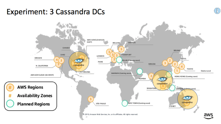
For this experiment, I used cqlsh running on my laptop, located in Canberra (close to Sydney). My initial goal was limited simply to explore latencies and try out failures of DCs. 

To measure latency I turned “tracing on”, and to simulate DC failures I created multiple keyspaces, connected cqlsh to different DCs, and used different consistency levels. 

I created three separate keyspaces for each DC location. This doesn’t result in data replication across DCs, but instead directs all data written to any local DC to the single DC with RF > = 1. I.e. All data will be written to (and read from) the DCSydney DC for the “Sydney” keyspace:

I used a fourth keyspace for replication. Because this has multiple DCs with RF >= 1 the data will be replicated across all of the DCs, i.e. data written to any local DC will be written locally as well as to all other DCs:

2.1 Latency

First let’s look at latency.  To run latency tests I connected cqlsh to the Sydney Data Center.

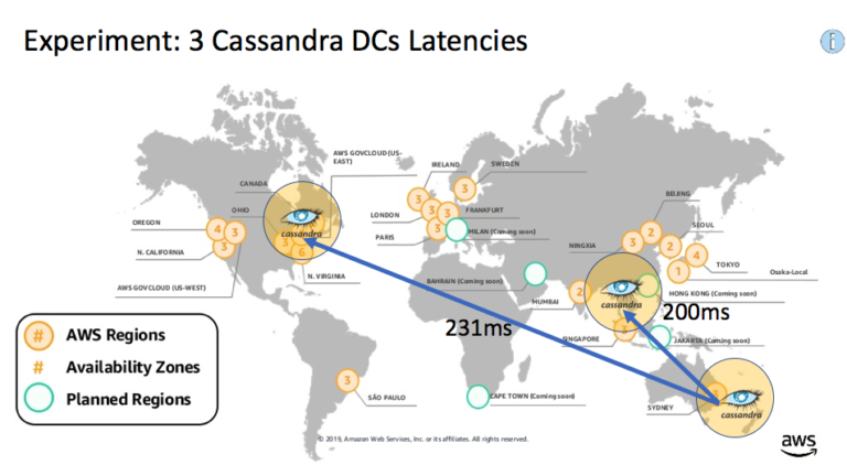
I varied which keyspace I was writing or reading to/from (Keyspace column), and used consistency level ONE for all of these. ONE means that a write must be written to and acknowledged by at least one replica node, in any DC, so we don’t expect any write/read errors due to writing/read in a local DC which is different to the DC’s in the keyspace. The results show that latency increases from a minimum of 1-2ms (Sydney), to 200ms (Singapore) and 231ms (USA). Compared to the average inter-region network latencies I reported in the previous blog these latencies are 14% higher—the Singapore latency is 200ms (c.f. 174ms), and the USA latency is 231ms (c.f. 204ms). Longer times are to be expected as there is a Cassandra write or read included in this time, on top of the basic network latency. As expected (using consistency ONE) all of the operations succeeded. This table shows the results:

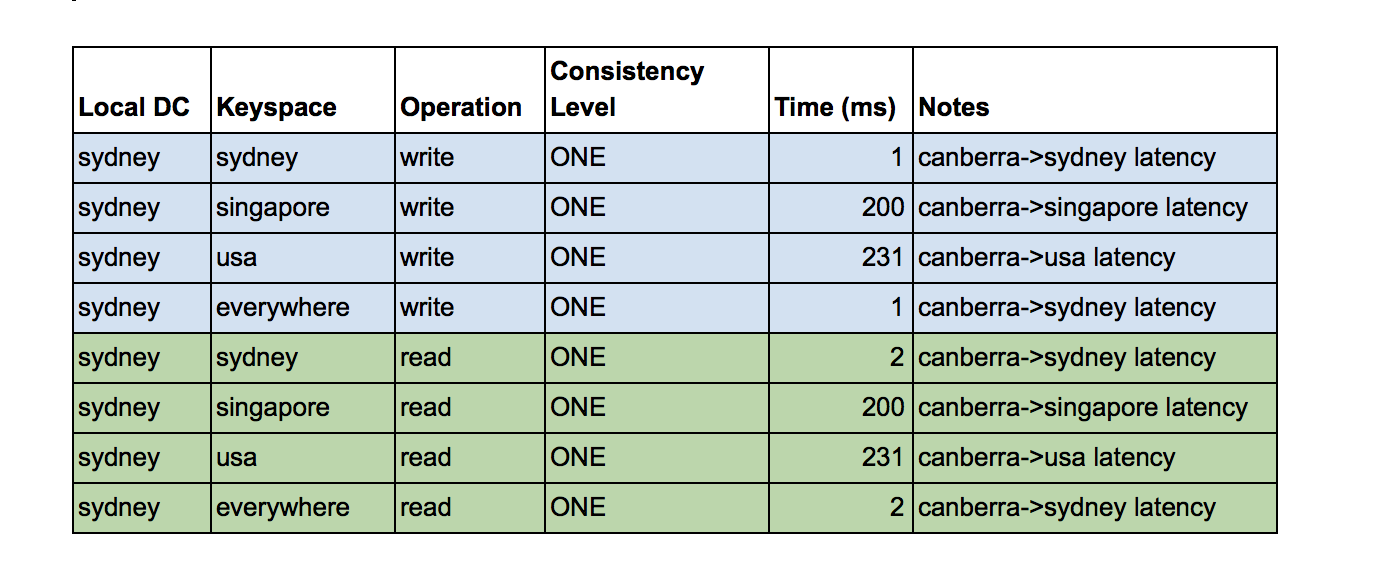
What does this reveal about how Cassandra keyspaces and DCs work? Cqlsh is connected to the Sydney DC as the local DC. For the keyspaces that just have a single DC, the write or read operation can only use that DC and therefore includes the overhead of network latency for the local DC to communicate with the remote DC (with no network overhead for sydney). However, for the “everywhere” keyspace which contains all three DCs, it behaves as if it’s just using the local DC and therefore has a low latency indistinguishable to the results for the “sydney” keyspace. The difference is that the row is written to all the other DCs asynchronously, which does not impact the operation time.  This picture shows the latencies on a map:

2.2 Failures

I also wanted to understand what happens if a DC is unavailable. This was tricky to achieve acting as a typical user for Instaclustr Managed Cassandra (as there’s no way for users to stop/start Cassandra nodes), so I simulated it by using permutations of local DC, keyspaces, and a consistency level of LOCAL_ONE (a write must be sent to, and successfully acknowledged by, at least one replica node in the local DC). This also allows customers to try this out as well. Using LOCAL_ONE means that if cqlsh is connected to the Sydney DC, and the keyspace has a Sydney DC with RF >= 1 then writes and reads will succeed. But if the keyspace only has DCs in other regions (Singapore or USA) then the writes and reads will fail (simulating the failure of remote DCs).  This table shows the results of this experiment:

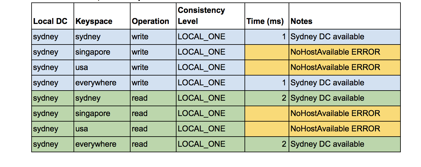
The results are almost identical to before, but with the key difference that we get a NoHostAvailable error (and therefore no latencies) when the keyspaces are Singapore or USA. The keyspace of Sydney or everywhere works ok still as the Sydney DC is available in both cases. 

Note that Cassandra consistency levels are highly tunable, and there are more options that are relevant to multi-DC Cassandra operation. For example, ALL and EACH_QUORUM (writes only) work across all the DCs, and have stronger consistency, but at the penalty of higher latency and lower availability.

3. Multi-Data Centers Experiments With the Cassandra Java Client

In our journey “Around the World” it’s important to always have the latest information, as Cassandra documentation can get out of date very quickly.

I was also interested in testing out the Cassandra Java client with my multi-DC cluster.   I had previously read that by default it supports automatic failover across multiple DCs which I thought would be interesting to see happening in practice. The DCAwareRoundRobinPolicy was recommended in the O’Reilly book “Learning Apache Cassandra (2nd edition 2017)” which says that “this policy is datacenter aware and routes queries to the local nodes first”. This is also the policy I used in my first attempt to connect with Cassandra way back in 2017!

However, a surprise was lying in wait! It turns out that since version 4.0 of the Java client there is no longer a DCAwareRoundRobinPolicy!  

Instead, the default policy now only connects to a single data center, so naturally, there is no failover across DCs. You must provide the local DC name and this is the only one the client connects to. This also means that it behaves exactly like the last (LOCAL_ONE) results with cqlsh. This prevents potentially undesirable data consistency issues if you are using DC-local consistency levels but transparently failover to a different DC.

You can either handle any failures in the Java client code (e.g. if a DC is unavailable, pick the backup Cassandra DC and connect to that), or probably the intended approach is for the entire application stack in the DC with the Cassandra failure to failover to a complete copy in the backup region. I tried detecting a failure in the Java client code and then failing over to the backup DC. This worked as expected. However, in the future, I will need to explore how to recover from the failure (e.g. how do you detect when the original DC is available and consistent again, and switch back to using it).

3.1 Redundant Low-Latency DCs

This brings us full circle back to the first blog in the series where we discovered that there are 8 geo regions in AWS that provide sub 100ms latency to clients in the same geo region:

The 8 AWS geo regions with sub 100ms latency for geolocated clients

Which we then suggested could be serviced with 8 DCs to provide DC failover in each geo region as follows:

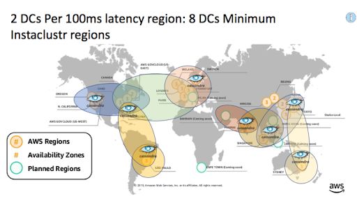
The matched pairs of DCs to provide High Availability (HA) and failover for each geo region look like this in table form. These are pairs of DCs that the application code will need to have knowledge of and failover between:

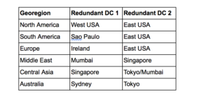
In practice, the read load of the application/client would need to load balance over both of the data centers for some geo regions (e.g. North America geo region load balances across both West and East Coast DCs). Depending on the data replication strategy (just replicating data written in each geo region to both redundant DC pairs, or to all DCs in the cluster—this really depends on the actual use case), and the expected extra load on each DC due to failover, DC cluster sizes will need to be sufficient to cope with the normal read/write loads on each DC, the replication write load (write amplification), and load spikes due to DC failures and failover to another DC. 

Based on these limited experiments we are now ready for the next Blog in the series, where we’ll try multi-DC Cassandra out in the context of a realistic globally distributed example application, potentially with multiple keyspaces, data centers and replication factors, to achieve goals including low latency, redundancy, and replication across geo regions and even Around The World.